Tutorial: from a crystal structure to a predicted spectrum

This tutorial starts with nothing but a crystal structure file and ends with a predicted spectrum for the VISION spectrometer at the Spallation Neutron Source, plus ready-to-edit inputs for the other two IRMA outputs. A pretrained machine-learned interatomic potential stands in for the first-principles calculation, so no DFT and no phonon calculation are needed up front. The material is the committed rocksalt MgO cell, examples/mlip/MgO.cif; after a one-time environment build, the whole chain runs in under a minute. You need the mlip and spectra extras (pip install -e ".[mlip,spectra]", see Installation).

Any structure file that ASE (the Atomic Simulation Environment, the library IRMA uses to read structures) can recognize from its name works in place of the CIF here; the naming rule (and its one failure mode) is spelled out at the top of MLIP phonon calculations.

One-time setup: the potential's environment

The pretrained potentials are never installed with IRMA, because their package stacks conflict with each other. Instead, each potential gets its own Python environment, built once:

The tutorial uses nequip, the potential that performed best in the validation snapshot; any of the nine works the same way.

irma mlip env create nequip

  building a dedicated environment for nequip ...
  create venv ...
  install requirements ...
  verifying `import nequip.ase` ...
  registered nequip -> ~/.cache/irma-mlip/envs/nequip/bin/python
  done; builds with --potential nequip now run in it automatically

The step is network-bound (it downloads the potential's package stack) and takes a few minutes. From then on, every irma mlip command detects the registered environment and runs nequip in it; nothing else needs activating.

Build the phonon calculation

irma mlip build examples/mlip/MgO.cif -o mgo_bundle --potential nequip

  relaxing with nequip (fmax=0.01 eV/A, nmax=100, cell=no)
  relaxation: converged=True fmax=2.27e-07 eV/A in 0 steps
  supercell (3, 3, 3), quick-look mesh (9, 9, 9)
  2 displacement(s), 216 atoms/supercell, jobs=1
  displacement 1/2 done
  displacement 2/2 done
  bundle written and validated: mgo_bundle

The build relaxes the structure with the potential, chooses a supercell, and runs the phonopy finite-displacement workflow with the potential supplying the forces. (The committed cell is already at nequip's minimum, so the relaxation converges in zero steps; your own structure will usually take tens of steps.) Rocksalt symmetry reduces MgO to two displacements, so this build finishes in 19 seconds on a laptop; lower symmetry means more displacements and proportionally more time. The bundle directory now holds the phonon calculation (phonopy.yaml), the relaxed cell (structure_relaxed.vasp), the build manifest, and the phonon density of states as both data (dos.dat) and a plot (dos.png). Look at dos.png before going further: a sensible DOS with no imaginary modes (imaginary modes plot as intensity at negative frequencies) is the cheapest sanity check the bundle offers, and the MLIP examples page shows what healthy and unhealthy ones look like.

Generate the three inputs

irma mlip emit mgo_bundle --to endf,spectra,ncrystal --mat Mg=45 --mat O=46

The --mat values are the ENDF material numbers the two evaluations will carry; they are yours to choose (any positive integer works for in-house use; libraries assign them by convention). The command prefills one input file per principal scatterer (endf_Mg.input, endf_O.input), a spectra configuration (spectra.yaml), and an NCrystal export configuration (ncrystal.yaml), and it prints the exact commands that run each one. The prefilled files carry the production settings: the same mesh density the validation campaign used (24x24x24 for this cell) and the full campaign sampling, so running them unedited gives production quality, not a quick approximation. The command also warns about anything it had to assume:

  Mg: natural element (za=12000); select an isotope with --nuclide Mg=<A>-Mg to take its identity AND its constants
  O: natural element (za=8000); select an isotope with --nuclide O=<A>-O to take its identity AND its constants

A phonopy calculation names elements, not isotopes, so each species is emitted as the natural element with that element's natural-abundance scattering constants. If your material is isotopically enriched, or you are evaluating a specific isotope, say so with --nuclide: it takes the ENDF identity and the constants from the same isotope entry, so the two cannot disagree (for example --nuclide Mg=26-Mg for magnesium-26).

Run the spectrum

irma spectra run mgo_bundle/spectra.yaml -o spectrum.csv

About twenty seconds later, spectrum.csv holds the mode-2 VISION spectrum at both detector banks:

# IRMA spectrum: geometry=vision mode=2 angles_deg=[45.0, 135.0] q_cuts=[] components=False elastic=True edges=13
E_meV,total@45deg,total@135deg
0,0.0062721171,0.0061556434
1,3.4521343e-05,3.4512376e-05

Plot the two bank columns to see the spectrum; with matplotlib:

import numpy as np, matplotlib.pyplot as plt
E, b45, b135 = np.genfromtxt("spectrum.csv", delimiter=",", skip_header=2).T
plt.plot(E, b45, label="45 deg"); plt.plot(E, b135, label="135 deg")
plt.xlabel("Energy transfer [meV]"); plt.legend(); plt.show()

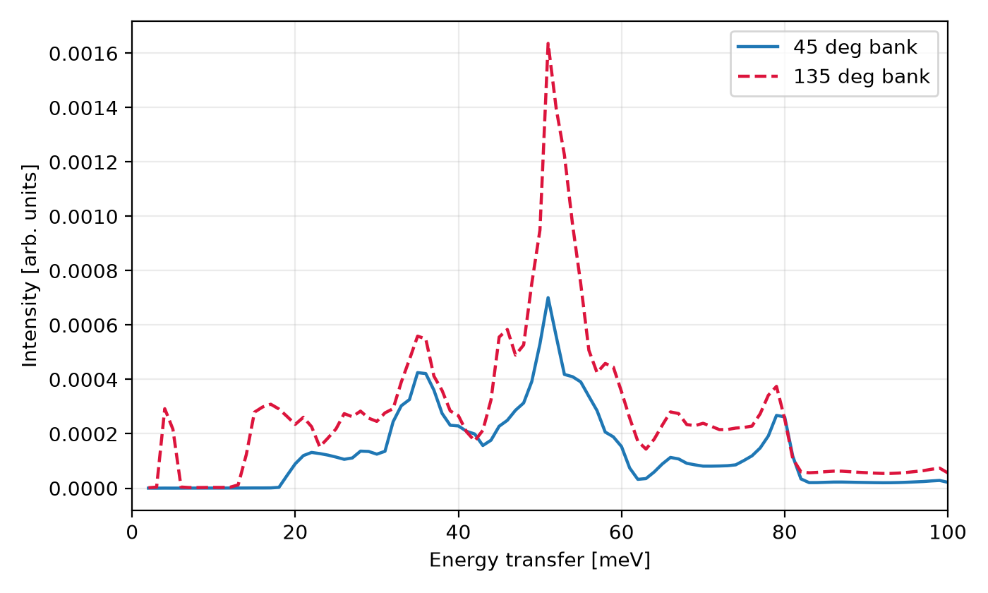
Three features stand out, and your plot should show all of them: an acoustic peak near 35 meV, the strongest optical peak near 51 meV, and a high-energy optical peak near 79 meV, with the one-phonon spectrum ending just above 80 meV (the small intensity beyond it is multiphonon scattering). The 135° bank sits higher than the 45° bank because its kinematics reach larger momentum transfer.

The spectra page documents everything the configuration can change: instrument geometry, resolution, temperature, energy grid, and the DOS-based mode 0 that needs no eigenvectors at all.

The other two outputs

The emitted input files run exactly like the ENDF tutorial: irma mgo_bundle/endf_Mg.input endf_Mg.endf produced a 5.0 MB tape in 198 seconds here, the log noting that the prefilled multiphonon order 100 already exceeded the 78 the grid required. The ncrystal.yaml is the subject of the transport tutorial.

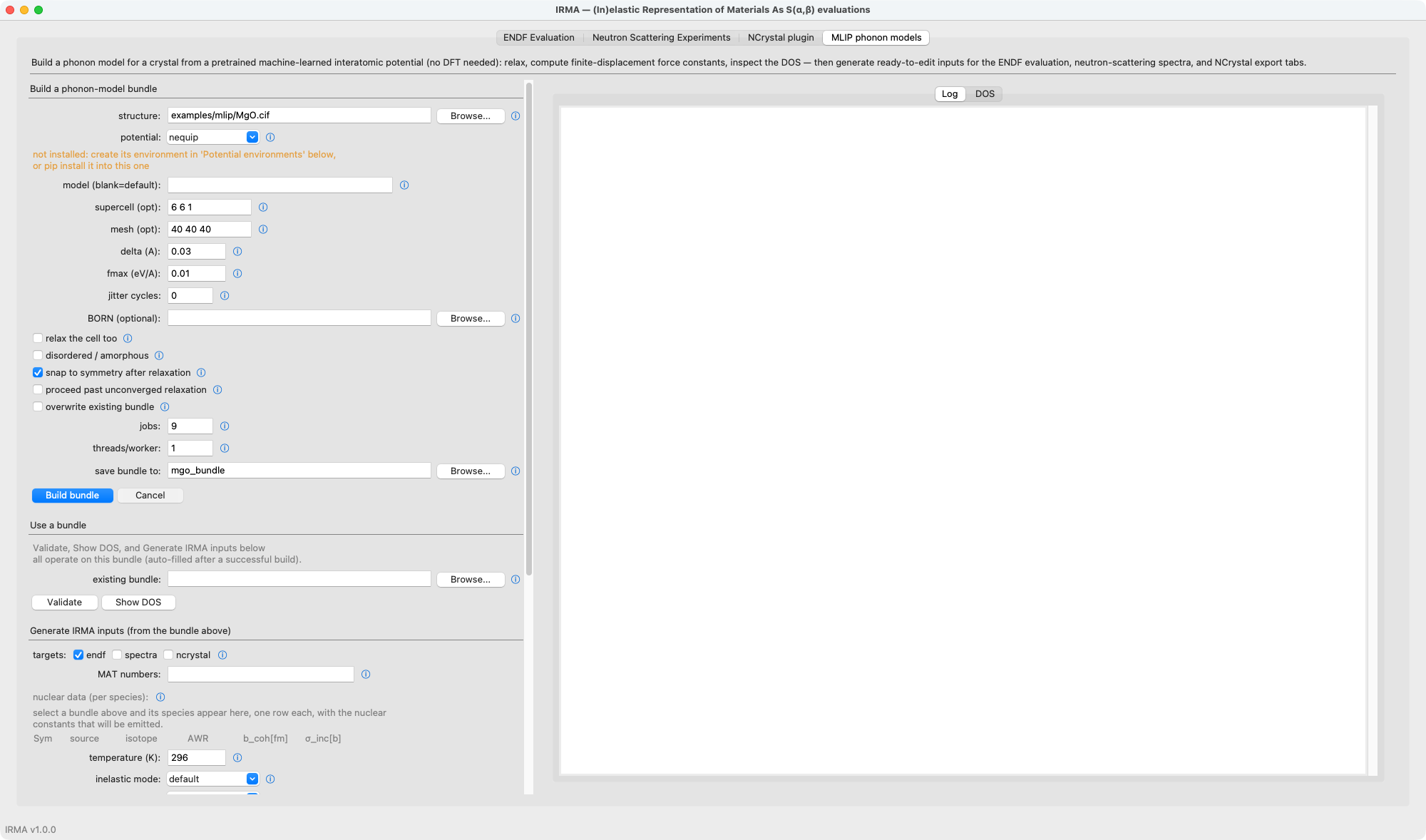
The same flow in the GUI

The MLIP phonon models tab is the build form: structure, potential, and every knob the CLI accepts, with the log and the DOS plot alongside. The "Generate IRMA inputs" section at the bottom is emit with checkboxes.