GUI guide

The IRMA graphical interface has four top-level tabs:

• ENDF Evaluation: a single-page front end for building a LEAPR-style input file (LEAPR is NJOY's thermal scattering law module, whose input format IRMA extends) and computing the thermal scattering law S(α,β) without hand-editing cards. The page is one scrolling form of five parts in the order the input file is written (Material, Scattering, Grids, Phonon, and Run) that you fill in top to bottom; the Jump to bar above the form scrolls any part to the top.
• Neutron Scattering Experiments: the forward-spectra panel; it predicts instrument-resolved INS spectra and 2-D S(Q,E) maps from a phonopy calculation or a phonon DOS, with no ENDF tape involved. Covered in its own section below.
• NCrystal plugin: exports the per-temperature material data file that the companion transport plugin samples on the fly. Covered in its own section below; the format and workflow are documented on the NCrystal data exporter page.
• MLIP phonon models: builds a bundle, a packaged phonon calculation, from a structure file with a pretrained machine-learned interatomic potential (MLIP) and generates ready-to-edit inputs for the other tabs. Introduced in its own section below; the full reference is the MLIP phonon calculations page.

The defining behavior of every tab is progressive disclosure: a field appears only when the mode that reads it is selected, so you never stare at controls that have no effect on your calculation. Importing an existing input file reveals exactly the sections it uses.

The second rule is what a fresh form does and does not claim: everything you should not have to think about is filled in, everything only you can know is empty. Method settings (mesh, ndir/mpdir, the automatic-grid knobs, the multiphonon order, the elastic format) ship at the recommended production values, so a first evaluation needs no tuning to be taken seriously. Material identity ships blank: ZA, MAT, AWR, sigma_free (all defined in the Scattering part below), the lattice parameters, the Card 6d atom types, and the per-element scatterer tables on the other tabs. IRMA cannot know your material, and a plausible-but-wrong prefill is worse than an empty field: someone evaluating BeO would see graphite's numbers, not recognize them, and ship a tape for the wrong material. Each blank group carries a gray hint naming the ways to fill it: Import Input File, a committed input file under examples/, Fill structure from phonopy.yaml (ENDF, modes 1/2), Fill AWR + sigma_free from ZA, or Auto-fill elements from phonopy.yaml (Neutron Scattering tab). This page describes each part in turn and calls out the pitfalls worth knowing before your first run.

Launching

irma-gui
# or
python -m irma --gui

The window title bar shows the product name, and the bottom bar shows the installed IRMA version.

How much of the form you see is decided by the modes you pick. Choosing iel=10 in the Material part unlocks the crystal-structure and phonopy sections; choosing inelastic_mode=1 or 2 unlocks the phonopy mesh and control fields and flags the legacy Phonon cards as not read; choosing a special mode (ncold, nsk, nss) in the Scattering part unlocks just that mode's extra inputs. Everything else stays hidden.

---

Material part

This is where you declare what you are modeling: the elastic treatment, and, for iel=10, the crystal structure and the noncubic inelastic mode.

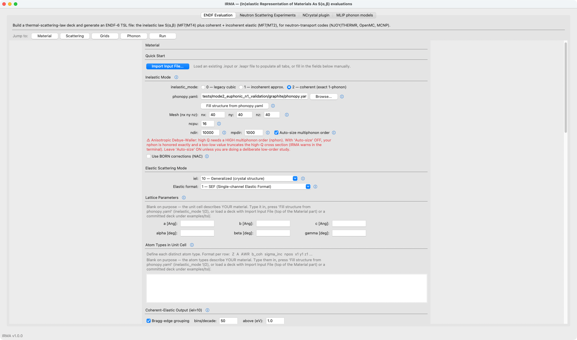
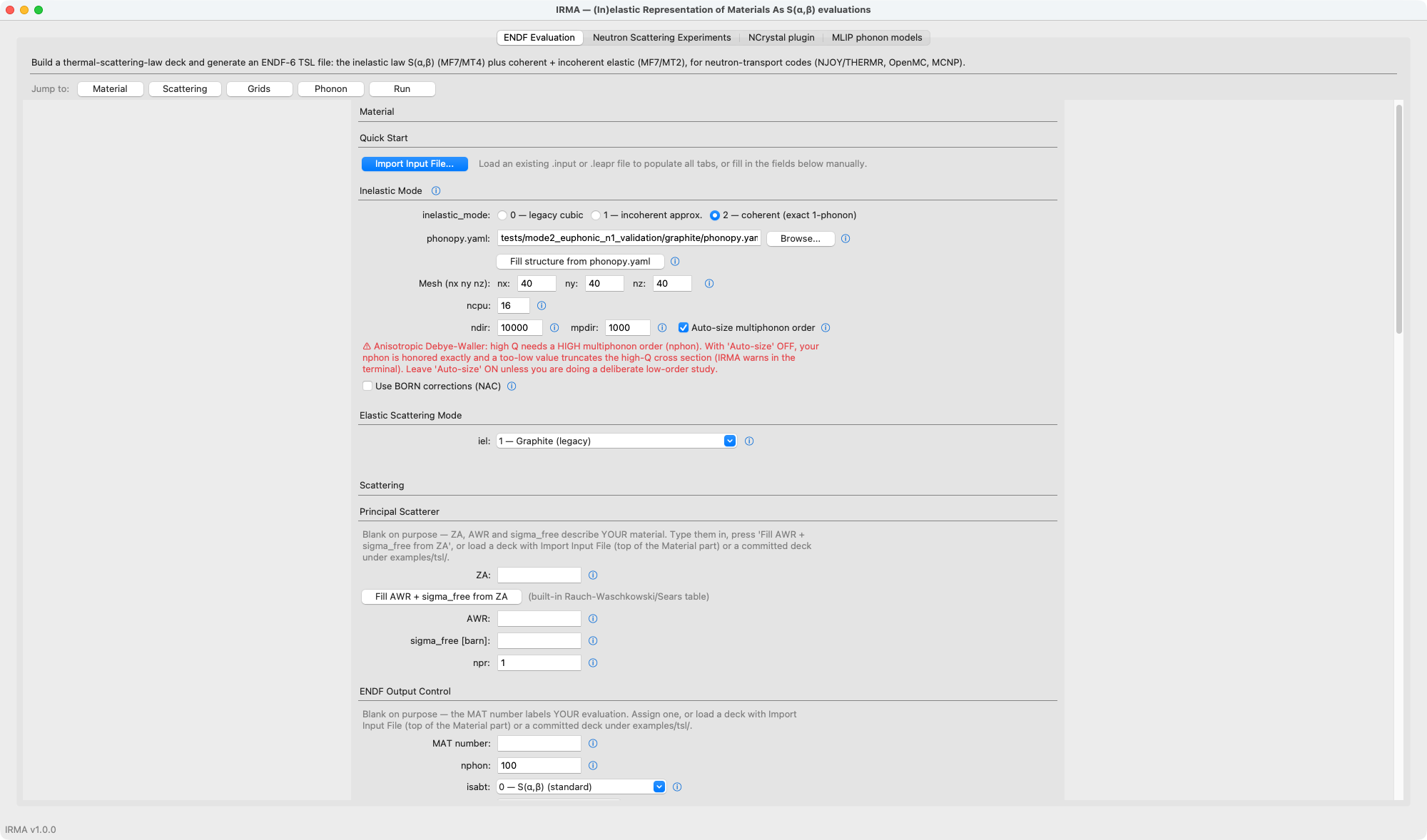
Progressive disclosure in action: with iel=10 and inelastic_mode=2, the lattice parameters, atom-type table, and the phonopy controls (mesh, ndir/mpdir, auto-size order, …) are all shown. Selecting a classic mode collapses them to a single dropdown:

Quick Start (input file import)

The Quick Start panel has a single Import Input File... button (also reachable from File ▸ Import Input File). Point it at an existing .input or .leapr input file and IRMA parses it and populates the whole form. Because import writes the same internal variables that your clicks do, the conditional sections reveal themselves automatically: an input file with iel=10 shows the crystal cards, one with a secondary scatterer shows the secondary fields, and so on. This is the fastest way to start from a known-good evaluation and tweak it. Import is optional: you can also fill in every field by hand; the button just saves typing.

Inelastic Mode (inelastic_mode)

This section chooses the inelastic model.

The inelastic_mode radio buttons:

inelastic_mode	Label	What it does
0	legacy cubic	Isotropic Debye-Waller, phonon expansion from a scalar DOS supplied in the Phonon part.
1	incoherent approx.	The inelastic part comes from the phonopy calculation with directional Debye-Waller factors, treating every atom as an incoherent scatterer (no interference between atoms).
2	coherent (exact 1-phonon)	The same, except the one-phonon term is exact: coherent interference between atoms is included. Multiphonon orders stay in the incoherent approximation. Matches the Neutron Scattering Experiments panel's "2 (coherent 1ph+multi)".

Modes 1 and 2 require the optional phonopy package, a phonopy.yaml with force constants, and the Card 6g controls below. They do not read the legacy continuous-DOS, translational, or oscillator cards in the Phonon part: MT4 and the directional elastic Debye-Waller factors come straight from the phonopy calculation. Selecting mode 1 or 2 reveals the phonopy sub-frame; mode 0 hides it.

Modes 1 and 2 are also defined only for iel=10, the generalized crystal-structure elastic treatment, so selecting one narrows the iel dropdown below to the generalized entry and switches the selection to it. Mode 0 restores the full iel list and leaves your selection alone. (Mode 0 is the legacy cubic treatment driven by the DOS you supply in the Phonon part, so it works with every iel; no phonopy is involved.)

Phonopy parameters (modes 1/2 only)

When inelastic_mode is 1 or 2, the sub-frame exposes:

Control	Default	Purpose
phonopy.yaml	—	Path to the phonopy YAML. Force constants are read from the YAML if embedded, otherwise discovered alongside it (force_constants.hdf5, FORCE_CONSTANTS, or FORCE_SETS).
Fill structure from phonopy.yaml	—	Button. Prefills the iel=10 Lattice Parameters and the whole Atom Types block from the phonopy.yaml named above, after a preview you confirm. See Atom Types.
Mesh nx ny nz	40 40 40	Monkhorst-Pack mesh for the Brillouin-zone sampling behind the directional (tensor) phonon DOS (matches the Neutron Scattering Experiments tab and the validation suite). Anisotropic crystals may use an asymmetric mesh.
ncpu	all cores	Parallel worker processes for the modes-1/2 workflow (prefilled with the machine's core count).
ndir	10000	One-phonon powder-average direction count: the validation-campaign sampling, well converged for production runs; drop to ~4000 for a faster look or ~1000 for a quick one. Cost is roughly linear.
mpdir	1000	Multiphonon powder-average directions over the unit sphere (golden-spiral / Fibonacci); converged by ~50–100, so the default carries ample margin.
Auto-size multiphonon order	on	When on (the default), IRMA sizes the multiphonon order nphon from the anisotropic Debye-Waller physics. When off, your Card 3 nphon is honored exactly (see below).
Use BORN corrections (NAC)	off	Non-analytical correction for polar materials; checking it reveals a BORN-file selector. Leave unchecked for non-polar materials such as graphite.

With the anisotropic Debye-Waller factor the multiphonon order needed to reach the free-gas limit grows with Q, so a hand-set nphon that is fine at low Q will silently truncate the high-Q rows of the cross section. With the default grids (Beta max = 5 eV, graphite AWR) the grid reaches Q ≈ 98 Å⁻¹, where an order near 223 is needed while the default nphon is 100. The GUI therefore ships Auto-size multiphonon order on. If you turn it off (a deliberate low-order study), IRMA honors your nphon exactly and prints a terminal warning when it is too low.

The multiphonon powder average converges quickly: for graphite-like crystals it is already converged by roughly 50–100 directions, so the default mpdir of 1000 is deep inside the converged regime. Cost scales linearly with mpdir, so larger values cost proportionally more without improving a converged result; raise it only to verify convergence on a new material.

The coherent one-phonon powder averaging always uses the golden-spiral direction quadrature; it is not user-selectable.

The GUI defaults produce Card 6g 10000 1000 1: 10000 coherent directions, 1000 multiphonon directions, auto-sized multiphonon order, the same sampling the validation campaign ran and irma mlip emit writes. (The powder averages converge well below these counts, so entering 4000 200 gives a faster exploratory run.)

Elastic Scattering Mode (iel)

The iel dropdown selects the coherent-elastic (Bragg-edge) treatment.

iel	Meaning
0	No coherent elastic scattering
1–6	Legacy built-in materials: graphite, Be, BeO, Al, Pb, Fe (hardcoded crystal structures)
10	Generalized: Bragg edges computed from the crystal structure you define in this part, for any material

iel=10 is the recommended option for new evaluations and is the default selection. It also unlocks the rest of the part: the Elastic format selector, Lattice Parameters, Atom Types, Coherent-Elastic Output, and Crystalline Extinction appear only for iel=10. For the built-in materials (iel=0–6) those cards are not read, so the GUI hides them to keep you from filling in fields that have no effect. The Inelastic Mode section above is not part of that group; it stays visible for every iel.

Elastic format (elastic_mode, iel=10 only)

elastic_mode	Format	Behavior
1	SEF (single-channel elastic format)	One ENDF-legal elastic section per tape: a single-atom material gets coherent elastic scaled by the full strength when sigma_coh > sigma_inc, else incoherent elastic carrying the sum; a polyatomic cell routes the designated-coherent atom (the one minimizing the incoherent contribution) to coherent elastic and redistributes the rest incoherently (Eq. 26 of the mixed-elastic paper, NIM-A 1027 (2022) 166227). See the theory page for the exact rule. Standard format, supported by all transport codes.
2	MEF (Mixed Elastic Format)	Every atom gets both coherent and incoherent elastic (LTHR=3). More accurate for polyatomic materials, but needs downstream transport-code support for the mixed format.

Lattice Parameters (iel=10 only)

Six fields define the unit cell: edge lengths a, b, c in Ångström and angles alpha, beta, gamma in degrees. They start blank (the cell is your material's identity, not something IRMA can guess) and are filled by hand, by Fill structure from phonopy.yaml (modes 1/2, below), or by importing an input file. Common settings:

• Cubic: a = b = c, alpha = beta = gamma = 90
• Hexagonal: a = b, alpha = beta = 90, gamma = 120

Atom Types (iel=10 only)

A free-text box, empty on a fresh form (like the lattice, the atom block is your material's identity), one line per distinct atom species, in the column order shown in the header:

Z  A  AWR  b_coh  sigma_inc  npos  x1 y1 z1  x2 y2 z2 ...

Field	Meaning
Z	Atomic number
A	Mass number
AWR	Atomic weight ratio to the neutron mass
b_coh	Coherent scattering length (fm)
sigma_inc	Incoherent cross section (barn)
npos	Number of equivalent positions in the cell
x y z ...	Fractional coordinates of each position

For a polyatomic material such as NaCl, use one line per species. Scattering lengths and cross sections come from the NIST neutron scattering-length tables.

Filling the structure from a phonopy calculation

For inelastic_mode 1 or 2 the Fill structure from phonopy.yaml button (under the phonopy.yaml selector) writes both the lattice fields and the whole atom block from the phonopy.yaml named on Card 6f. The cell it reads is the phonopy primitive cell, loaded through phonopy itself: the cell those modes require, since IRMA matches every Card 6d position against the phonopy primitive cell's atom positions and refuses an input file whose positions do not correspond.

The button never fires on its own: not when you select a phonopy.yaml, not on input-file import, not on reset. It opens a preview of the exact lattice line and atom rows it would write; Apply replaces both together, Cancel changes nothing, so phonopy positions can never end up beside a hand-typed lattice.

Each species is filled as the natural element: ENDF codes that as A = 0, and AWR, b_coh and sigma_inc are that element's natural-abundance values, so the identity and the constants always come from one table entry. A phonopy calculation names elements, not isotopes: it typically labels deuterium as H and says nothing about enrichment, so an isotopic or enriched material must be edited afterwards. Elements whose tabulated scattering length is a resonance-region (energy-dependent) value are refused rather than prefilled.

Cells that are not in Ångström are converted, not refused. phonopy keeps cells in the calculator's native length unit and does not convert them on load, so a calculation built through the qe, abinit, elk, siesta, wien2k, DFTB+, TURBOMOLE, fleur, abacus or qlm interface carries a cell in bohr. IRMA applies the calculator's factor once, at load, in the same place inelastic_mode 1/2 does, so the lattice this button writes is the lattice the engine runs. A phonopy.yaml is refused only when its length unit is genuinely unusable: a physical_unit: length: name IRMA cannot map to a factor, or a calculator interface missing from phonopy's own units table.

Coherent-Elastic Output (iel=10 only)

The Bragg-edge grouping controls live in their own frame between the atom-type table and the phonopy section, because they are a coherent-elastic MF7/MT2 output option that applies to every iel=10 inelastic mode, including the classic mode 0, which needs no phonopy at all.

The Bragg-edge grouping checkbox is on by default (compact tapes); uncheck it to keep every Bragg edge. When checked, two fields control the grouping of dense high-energy edges, following ENDF-102 §7.2.2. Importing an input file sets the checkbox to match it (on only if it carries the Card 6b grouping fields).

Field	Default	Meaning
Bragg-edge grouping (checkbox)	on	Group dense high-energy edges. Uncheck to write every edge (the former default).
bins/decade	50	Above the threshold, the energy axis is split into this many log-uniform bins per decade; all edges in a bin merge into one step at the structure-factor-weighted log-mean energy.
above (eV)	1.0	Energy above which grouping may occur. Edges at or below it are always kept individually.

Grouping preserves the cumulative edge sum (the running total of Bragg-edge strengths), the total bound cross section, and the high-energy 1/E tail; only the placement of merged high-energy steps is approximate (IRMA prints the resulting integral cross-section error per temperature). These map to optional fields 5–6 on Card 6b. Grouping composes with extinction: extinction refines the Bragg edges below ~0.1 eV while grouping compacts those above the threshold.

Crystalline Extinction (iel=10 only)

The Crystalline Extinction (Optional) frame applies a dynamical-diffraction reduction to the coherent-elastic Bragg edges, the effect that makes a real crystallite's peaks weaker than ideal theory predicts. It is a specimen property, off by default.

Tick Enable extinction correction and the parameter fields appear (hidden while the correction is off): pick a model (five available; the coupled BC_mix/BC_mod need l, g, and L all > 0), and set the specimen sizes: l (crystallite, primary), g (mosaic) and L (grain) for secondary, plus the distribution, recipe, and tabulation rmse_tol. Every control has an ⓘ help glyph (hover for a preview, click for the full text) explaining the parameter and linking the references; the attribution line credits the NCrystal CrysXT plugin. Changing the model snaps the distribution to that model's default (Gauss for Becker-Coppens, rect for Sabine). The section round-trips through input-file export/import.

See Crystalline extinction for the full physics, the extinction card, validation, and references.

---

Scattering part

Here you describe the principal scatterer, control the ENDF output, and opt into any special moderator physics.

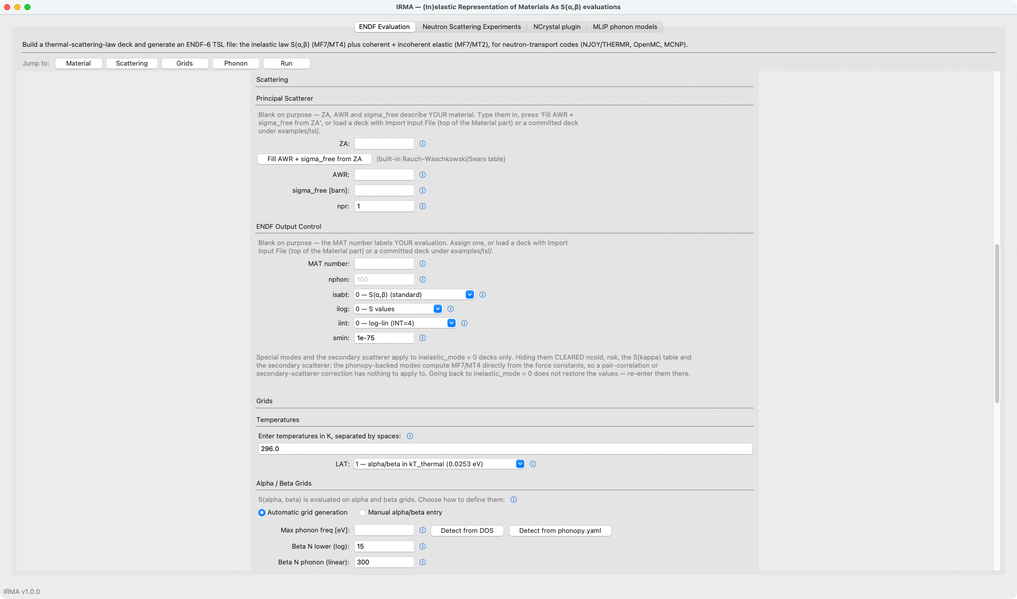
Principal Scatterer

The first three fields are material identity and ship blank; npr is a convention and does not.

Field	Default	Meaning
ZA	(blank)	Scatterer identity as Z×1000 + A, with A = 0 naming the natural element (6000 = natural carbon). Must match an atom type from the Material part.
AWR	(blank)	Atomic weight ratio to the neutron mass; drives recoil kinematics and alpha-grid scaling.
sigma_free (spr)	(blank)	FREE-atom scattering cross section (barn), exactly as on LEAPR Card 5. IRMA derives the bound cross section that normalizes S(α,β) internally as sigma_b = sigma_free·((1+AWR)/AWR)² and writes npr·sigma_free into the tape's B(1) field (an ENDF bookkeeping value). Do not enter the bound value (carbon: enter 4.739, not 5.55; hydrogen: enter ~20.45, not ~82; the bound value makes every MT4 cross section ~4× too large for H).
npr	1	Number of principal scattering atoms in the compound, not in the unit cell (≥ 1). For iel=1–6 it also scales the built-in Bragg-edge cross sections.

The Fill AWR + sigma_free from ZA button looks the ZA up in IRMA's built-in nuclear table (the Rauch–Waschkowski/Sears compilation, see irma.core.nuclear_data) and overwrites AWR and sigma_free with the tabulated values; sigma_free is derived from the bound cross section as sigma_b·(AWR/(1+AWR))², so the free/bound convention is always right. It is the quickest way out of the blank identity fields: type a ZA, press the button, and the other two follow. Pressing it with ZA still empty says so and changes nothing. Nuclides with energy-dependent scattering lengths (B, Cd, Gd, …) and isotopes without measured constants are refused with a message; enter those by hand.

Each input file evaluates one principal scatterer: for inelastic_mode=1/2, IRMA writes one principal-scatterer MT4 section per input file even when the crystal has several atom types. If you need more than one principal (for example Be and O in BeO), run separate input files.

ENDF Output Control

Field	Default	Meaning
MAT number	(blank)	ENDF material number for the output library; it labels your evaluation, so it is blank until you assign it or import an input file.
nphon	100	Maximum phonon expansion order. Light scatterers (H, D) reach much larger α for the same β grid and generally need more terms; heavy scatterers converge with fewer. For modes 1/2 this is also the multiphonon maximum order (unless Auto-size is on, the GUI default).
isabt	0 — S(α,β)	Which form of S(α,β) is stored. 0 is the standard symmetric S(α,β) required by THERMR; 1 writes the asymmetric S̃ form (diagnostics only, not for library production).
ilog	0 — S values	Storage form. 0 stores S directly; 1 stores ln(S) (ENDF LLN=1), useful when the table spans many decades and the processor supports it.
smin	1e-75	S(α,β) values below this threshold are treated as zero (LEAPR convention).

Special Modes

These selectors stay collapsed by default; choosing a non-zero value reveals only that mode's extra inputs.

Selector	Options	Reveals
ncold	None / Ortho-H / Para-H / Ortho-D / Para-D	The S(κ) table (dka, S(κ) values) when non-zero.
nsk	None / Vineyard / Sköld	The S(κ) table, plus cfrac (coherent fraction) when non-zero.

The S(κ) inputs (dka grid spacing and the space-separated S(κ) values) appear whenever nsk > 0 or ncold > 0. For nsk > 0 you must also give cfrac.

Neither selector is available with the phonopy modes: ncold and nsk are rejected with inelastic_mode=1/2, because MT4 comes from the phonopy calculation rather than a tabulated pair-correlation treatment. Selecting inelastic_mode=1 or 2 therefore hides the Special Modes and Secondary Scatterer sections and clears them: ncold, nsk, the S(κ) table and the whole secondary scatterer go back to their off values, so the rejected combination cannot be reached from the form at all. Switching back to inelastic_mode=0 does not restore the values; re-enter them there. A hand-written input file that carries the combination is still refused by the parser.

Secondary Scatterer (optional)

Set nss to 1 — One secondary scatterer to reveal the secondary-species fields:

Field	Meaning
b7	Secondary model: 1 free gas (most common, e.g. O in H₂O), 2 diffusion, 0 bound two-pass (the secondary gets its own phonon-spectrum pass, e.g. O in BeO).
AWS	Secondary atomic weight ratio (> 0).
sigma_s	Secondary free-atom cross section in barn (> 0).
mss	Number of secondary atoms in the unit (≥ 1).

Choosing b7 = 0 also reveals the Secondary phonon model (b7 = 0 two-pass only) panel (its own DOS spacing/values, translational weights, and oscillator energies/weights), which IRMA emits as a complete second pass through the temperature block (the secondary species' own spectrum and weights) and merges with bound-cross-section weighting. The two-pass merge exists only with the classic elastic options: with generalized elastic (iel = 10) a bound b7 = 0 secondary is rejected at parse time (use b7 = 1/2 or nss = 0).

For most polyatomic materials, evaluators generate a separate table per species (nss = 0) instead of using the mixed-moderator approach. A secondary scatterer is not supported with inelastic_mode=1/2, and combining ncold/nsk with the two-pass case is input-file-only.

---

Grids part

This part defines the temperatures and the α/β grids on which S(α,β) is tabulated (α and β are the dimensionless momentum and energy transfer; β = E/kT).

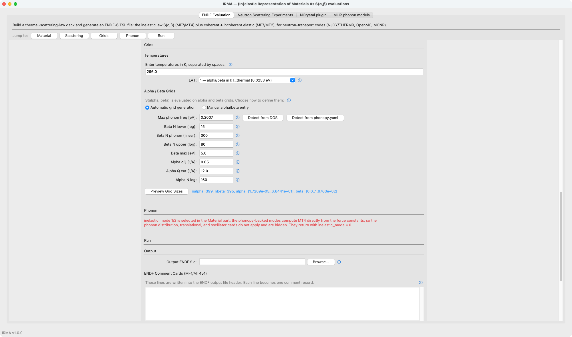
With Automatic grid generation selected, Preview Grid Sizes reports the resulting point counts and ranges without running the calculation.

Temperatures

Enter temperatures in Kelvin, space-separated. The phonon spectrum is read only at the first temperature; subsequent temperatures reuse it and recompute S(α,β) for the new Boltzmann population.

The LAT selector controls α/β scaling:

LAT	Meaning
0	α/β in units of kT = k_B·T (grid meaning changes per temperature).
1	α/β in units of a fixed kT_thermal = 0.0253 eV (T = 293.6 K). Standard ENDF TSL convention; the same grid serves all temperatures. Recommended (default).

Alpha and beta grids: automatic vs manual

A radio pair switches between Automatic grid generation (default) and Manual alpha/beta entry; only the chosen mode's fields are shown.

Automatic beta controls

The beta grid has three regions: a logarithmic low-β tail, a linear phonon region over [0, freq_max], and a logarithmic high-β tail up to Beta max.

Field	Default	Meaning
Max phonon freq	0.20	Upper bound of the linear region (eV). The Detect from DOS and Detect from phonopy.yaml buttons fill this in for you.
N lower (log)	15	Logarithmic points in the low-β (thermal quasi-elastic) tail.
N phonon (linear)	300	Linear points across [0, freq_max], where phonon features live.
N upper (log)	80	Logarithmic points in the high-β multiphonon tail. 80 is conservative: it keeps the high-β step fine enough that lin-lin (INT=2) interpolation does not overshoot the free-atom limit at high incident energy. Fewer (~20) suffice for log-lin or thermal-only runs; verify grid convergence for your energy range and adjust up or down.
Beta max	5.0	Maximum energy transfer (eV) for the upper tail. Hydrogen may need 10 eV or more.

Automatic alpha controls

The alpha grid is linear in momentum transfer Q: points every dQ out to Q cut, then a logarithmic tail to the beta grid's kinematic reach (α_max = 4·beta_max/AWR).

Field	Default	Meaning
Alpha dQ	0.05	Q spacing (1/Å) of the linear segment; α = Q²·(ℏ²/2m)/(AWR·kT). Sets how well the thermal upscatter windows (Q ≈ 1–6 1/Å) are resolved.
Alpha Q cut	12.0	Q (1/Å) where the grid switches from linear to a logarithmic tail. Fixed by neutron kinematics, not the material; rarely needs changing.
Alpha N log	160	Logarithmic points from Q cut to the grid maximum (feeds the epithermal cross section and the free-gas limit).

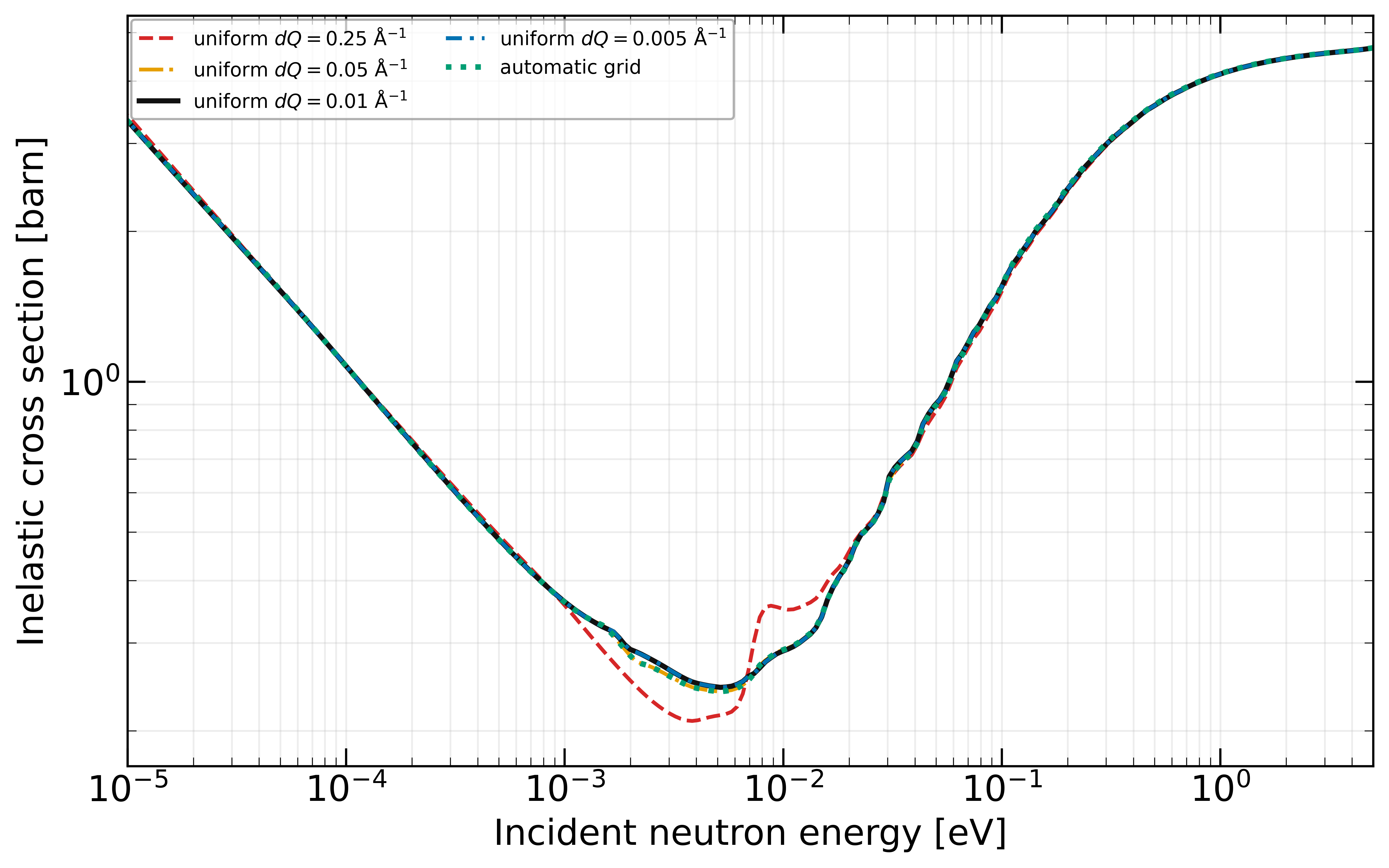
The linear-in-Q layout exists because the thermal-energy inelastic cross section integrates S(α,β) over upscatter windows at small α (Q ≈ 1–6 1/Å): an alpha grid that simply mirrors the beta layout under-integrates that cross section by 10–20%. On graphite at 296 K the default dQ = 0.05 grid lands within 3–5% of the converged result at only ~400 columns; a linear dQ = 0.01 grid is converged (halving dQ again moves results ≤0.3%).

Manual entry

Two text boxes take space-separated α and β values, both ascending; the β list should start at 0. Use this to match a reference evaluation exactly or to control grid placement precisely.

Preview

The Preview Grid Sizes button reports the resulting nalpha and nbeta (and the α/β endpoints in auto mode) without running the calculation, a quick sanity check on grid budget before you commit. The alpha and beta point counts are decoupled, so you can resolve the thermal Q window densely without inflating the energy grid.

---

Phonon part

This part supplies the scalar phonon input used by the legacy cubic treatment (inelastic_mode = 0). When inelastic_mode = 1 or 2 is selected in the Material part, the phonon distribution, translational, and oscillator sections disappear and a note explains why: modes 1 and 2 compute MT4 directly from the force constants and never read these cards. Selecting inelastic_mode = 0 (or a classic iel) brings the sections back.

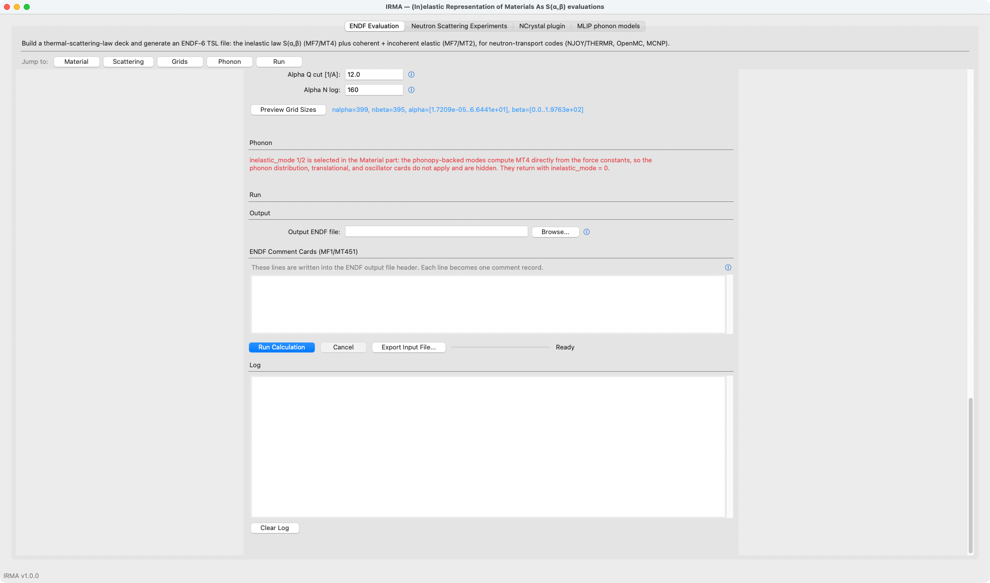
Continuous Phonon Distribution

A radio pair chooses the DOS source, and only the selected source's fields appear directly beneath its button:

• From phonopy total_dos.dat (default) — a file selector for a phonopy total_dos.dat (two columns: frequency in THz and DOS). IRMA converts THz→eV and normalizes the spectrum.
• Manual entry: delta_e (uniform energy spacing, eV) plus a space-separated rho list on the equidistant grid starting at E = 0.

Translational Mode

Field	Default	Meaning
twt	0.0	Weight of the translational (diffusive/free-gas) component. 0 for a crystalline solid.
c (diffusion)	0.0	Diffusion constant; 0 is free-gas translation, > 0 is the Egelstaff-Schofield diffusion model. Used only when twt > 0.
tbeta	1.0	Weight of the continuous distribution. The weights satisfy tbeta + twt + Σ(oscillator weights) = 1.

Discrete Oscillators

Two text boxes take space-separated oscillator energies (eV) and weights for isolated vibrational modes treated analytically, typically intramolecular modes such as the H₂O bend and stretch. Leave them empty for most crystalline solids.

---

Run part

The final part sets the output destination, optional ENDF documentation, and launches the job.

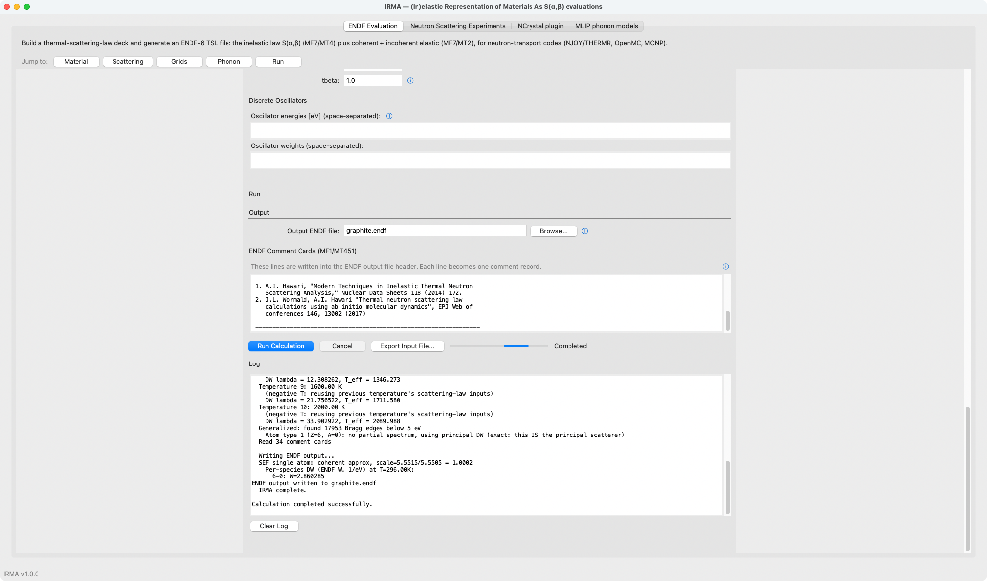
• Output ENDF file: destination for the ENDF-6 tape (S(α,β) in MF7/MT4, plus MF7/MT2 Bragg edges when iel > 0). This tape is what NJOY's THERMR and ACER modules process downstream into transport-ready data.
• ENDF Comment Cards (MF1/MT451): free-text box; each line becomes one comment record (truncated to 66 characters). Document the method and references here.
• Run Calculation: generates the input file from the current fields and runs it, streaming progress into the Log pane with an indeterminate progress bar, a status label, and a live phase readout showing the engine's current stage. Cancel terminates a running calculation; Clear Log empties the pane.
• Export Input File...: writes the generated input file to a .input/.leapr file without running, so you can inspect, archive, or hand it to the command-line tool.

Coherent mode-2 tapes need a stock-NJOY THERMR patch

A coherent inelastic_mode = 2 tape (graphite and similar) processed through unpatched NJOY2016 THERMR comes out as ~1e91-barn garbage above ~0.27 eV, or stalls for hours. This is a cliq bug in stock thermr.f90 (its guard tests decay along alpha but not beta), not an IRMA tape defect, and it fires on the shape of S(α,β), not its grid spacing, so no beta-grid choice avoids it. Apply the one-line two-axis guard patch first; inelastic_mode = 0/1 tapes and most materials are unaffected. See NJOY interoperability.

---

Neutron Scattering Experiments tab

The second top-level tab is the forward-spectra panel. It answers a different question than the ENDF Evaluation tab: that tab computes S(α,β), while this panel predicts what your instrument would measure, either an instrument-resolved 1-D INS spectrum or a 2-D S(Q,E) powder map, computed directly from a phonon calculation with no ENDF tape involved. It is the GUI face of the irma spectra command line; Save Config... / Open Config... round-trip the same YAML files the CLI runs, so you can prototype in the GUI and script the production run.

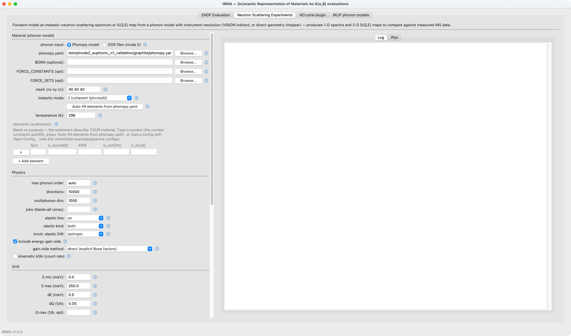
Material (phonon input)

The first control, phonon input, gates the whole panel:

• Phonopy model (default): point phonopy.yaml at your phonopy file (force constants are discovered next to it, or set FORCE_CONSTANTS / FORCE_SETS / BORN explicitly) and choose the mesh. Auto-fill elements from phonopy.yaml populates the element table with the cell's species and multiplicities.
• DOS files (mode 0): the route with no phonopy; each element row carries its own 2-column phonon DOS file (frequency, intensity; meV/eV/cm⁻¹/THz) instead. See DOS-based spectra (mode 0).

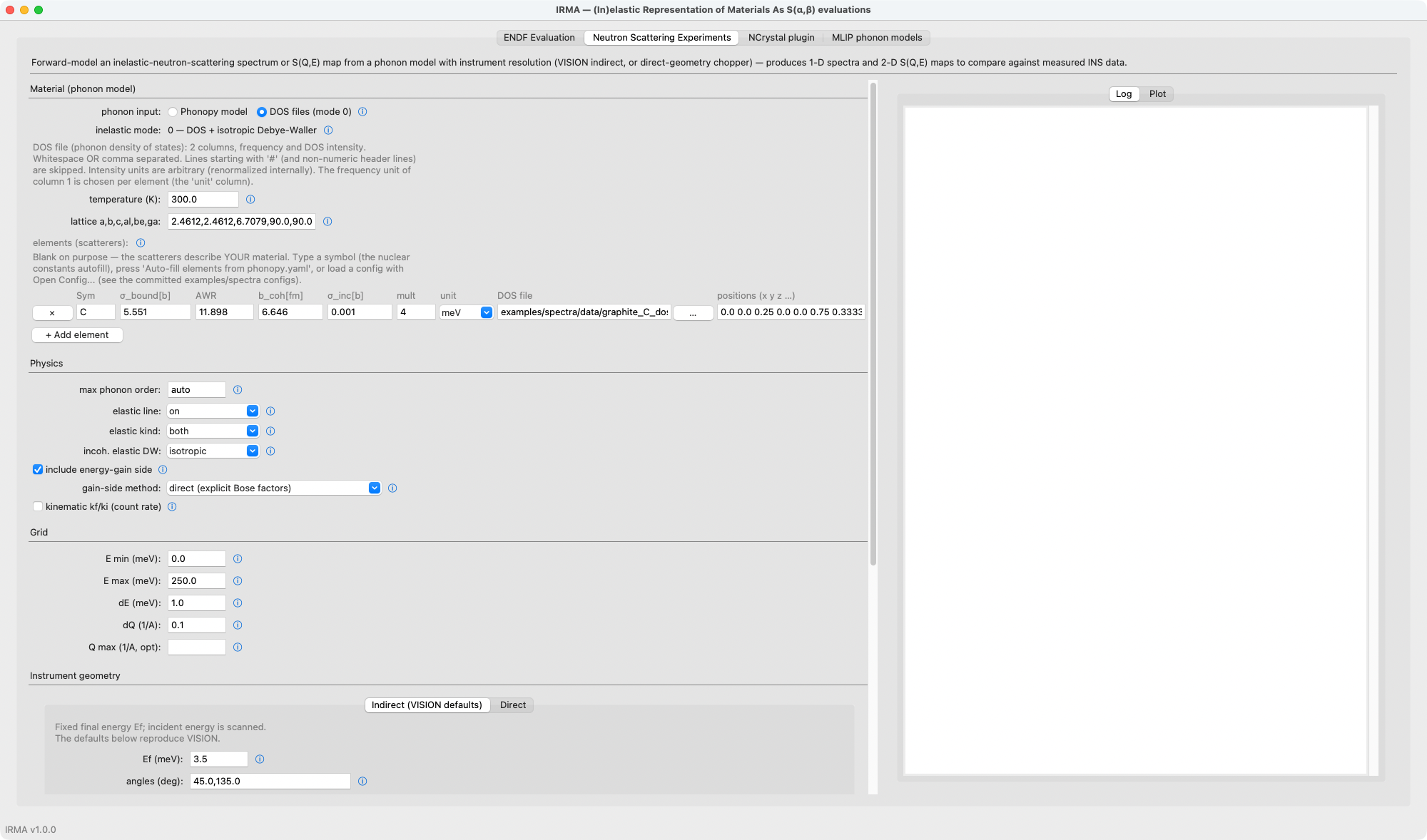
Below the gate sit the inelastic mode (0 DOS + isotropic Debye-Waller, 1 incoherent approximation, 2 exact coherent one-phonon; modes 1/2 need the phonopy input), the temperature, the optional lattice (needed only for the mode-0 coherent-elastic line), and the per-element table: symbol, σ_bound, awr, b_coh, σ_inc; plus, in DOS-files mode, the multiplicity, DOS file and frequency-unit columns, and, whenever a mode-0 elastic line is requested, the fractional positions column (flat x y z x y z …, as in an ENDF input file).

The table starts as one empty row: the scatterers name your material, so IRMA declares none of them. Typing a symbol (Be, O, …) and leaving the cell autofills the still-empty nuclear columns from IRMA's built-in table (irma.core.nuclear_data, the Rauch–Waschkowski/Sears compilation); anything you typed yourself is never overwritten, and typing a new symbol over a machine-filled row refreshes the prefilled constants. Nuclides with energy-dependent scattering lengths (B, Cd, Gd, …) are left blank on purpose: enter constants appropriate for your energy range by hand. Auto-fill elements from phonopy.yaml draws from the same table, and the NCrystal-plugin tab's element table behaves identically. Isotope labels (C-13, D, …) autofill too, but keep them for the DOS-files mode where the symbol is a free label: phonopy-backed modes and the NCrystal export match rows to the structure's chemical species by exact symbol, so an enriched material there needs the bare element symbol with hand-entered isotope constants.

Physics, Grid, and the elastic line

Physics holds the engine controls: max phonon order (auto recommended), and for modes 1/2 the powder-average directions, multiphonon dirs, and worker jobs, plus the elastic line switch, elastic kind (both, coherent, incoherent), and two toggles: include energy-gain side (anti-Stokes by detailed balance, on by default) and kinematic kf/ki (multiply by the flux factor to get the double-differential cross section, off by default). The elastic line is computed directly, with no ENDF file involved, from the same Debye-Waller factors as the inelastic part. Grid sets the energy window (E min/E max/dE) and the powder-average Q resolution (dQ), with an optional Q max cap.

Instrument geometry and resolution

Two sub-tabs select the geometry:

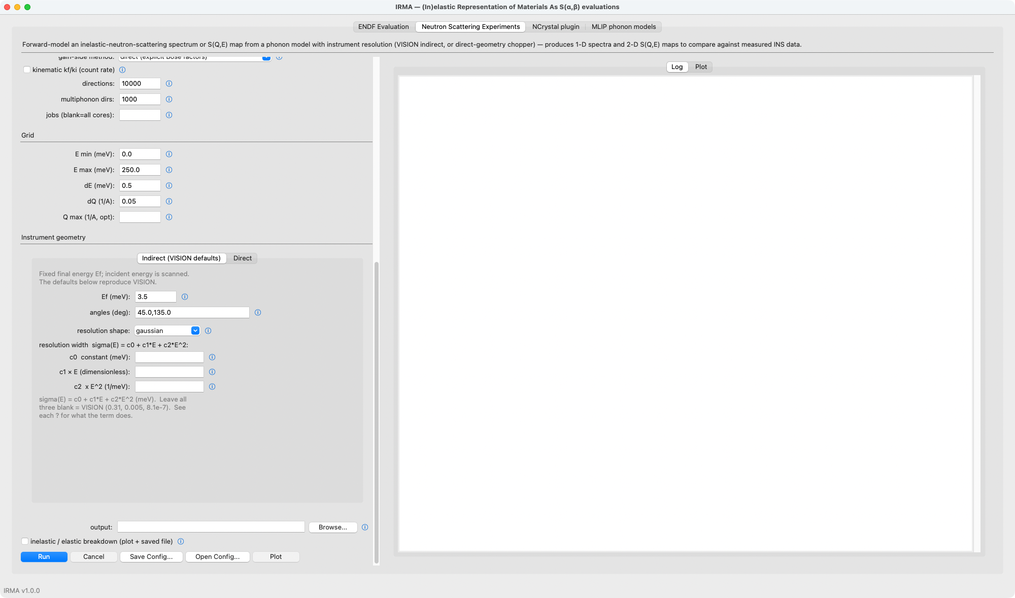
• Indirect (VISION defaults): fixed final energy Ef; the VISION preset fills Ef = 3.5 meV and the 45°/135° banks, or enter your own angles.
• Direct: fixed incident energy Ei plus an output selector: fixed cuts (cut by detector angles or constant-Q values, with an optional cut dQ band average) or a 2-D S(Q,E) map masked to the instrument's detector coverage 2θ arch.

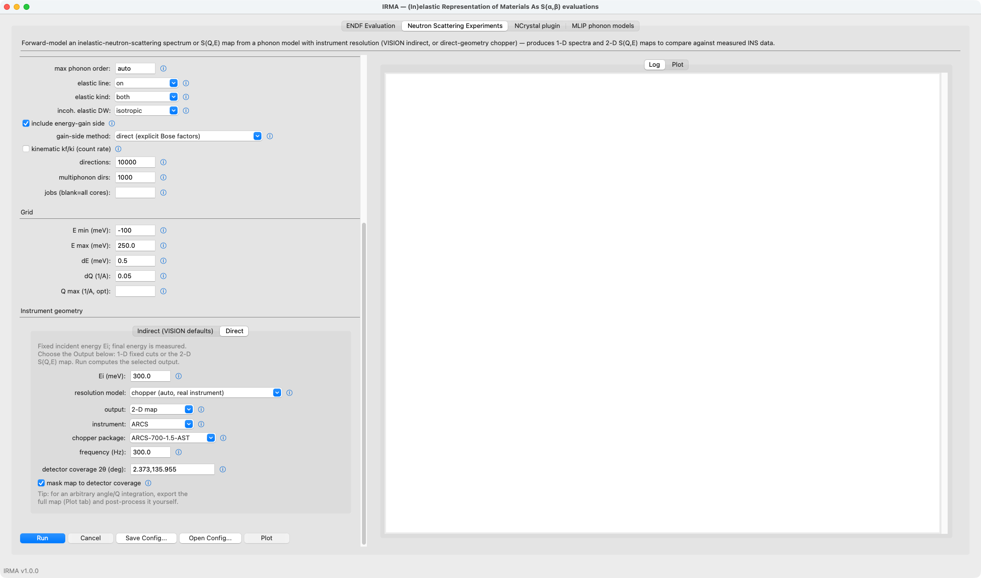
The resolution model is either a width polynomial (three labeled coefficients, sigma(E) = c0 + c1·|E| + c2·E² (meV), mirrored on the energy-gain side) or the automatic chopper model: pick the instrument (ARCS, SEQUOIA, MAPS, MARI, MERLIN, HYSPEC, CNCS, LET), the chopper package, and the frequency, and the energy-dependent width is computed for you (validated against Mantid PyChop to ~1%). resolution shape chooses Gaussian or Lorentzian.

The chopper model is an independent BSD reimplementation written from the published resolution literature; no PyChop (GPL) source is included. PyChop is the black-box validation reference and the collected source of the factual instrument parameters; see THIRD_PARTY_NOTICES.md in the repository for the full provenance statement.

Running and plotting

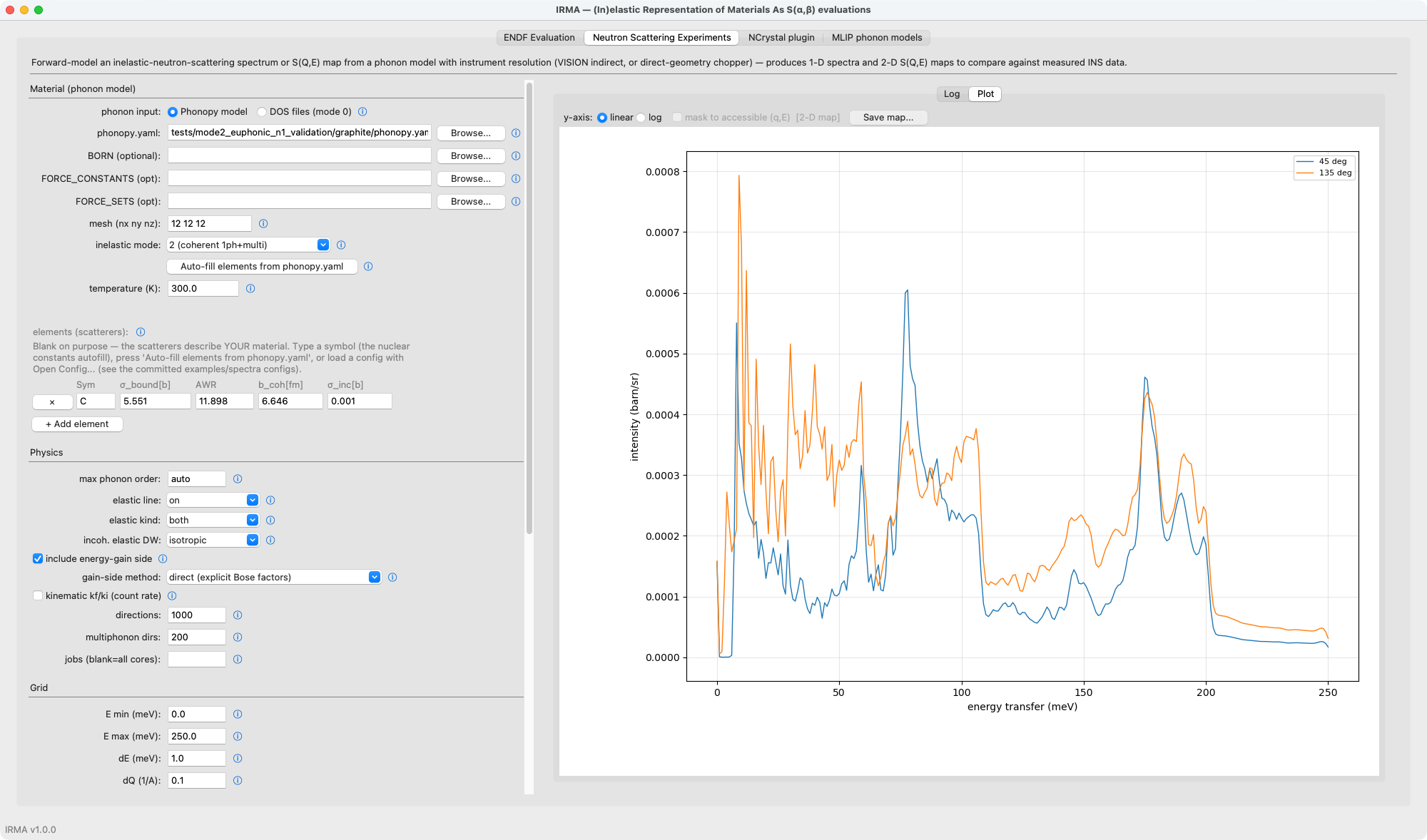
Run streams progress into the Log pane and enables Plot when done: spectra plot per-bank/per-cut curves (linear or log y-axis), maps render with the kinematic envelope and a mask to accessible (q,E) toggle, and Save map... exports the 2-D map to CSV/npz. The spectrum itself is written to the output path (CSV, npz, or JSON by extension); the inelastic / elastic breakdown toggle next to it keeps each cut's component columns in the saved file and overlays them on the 1-D plot.

---

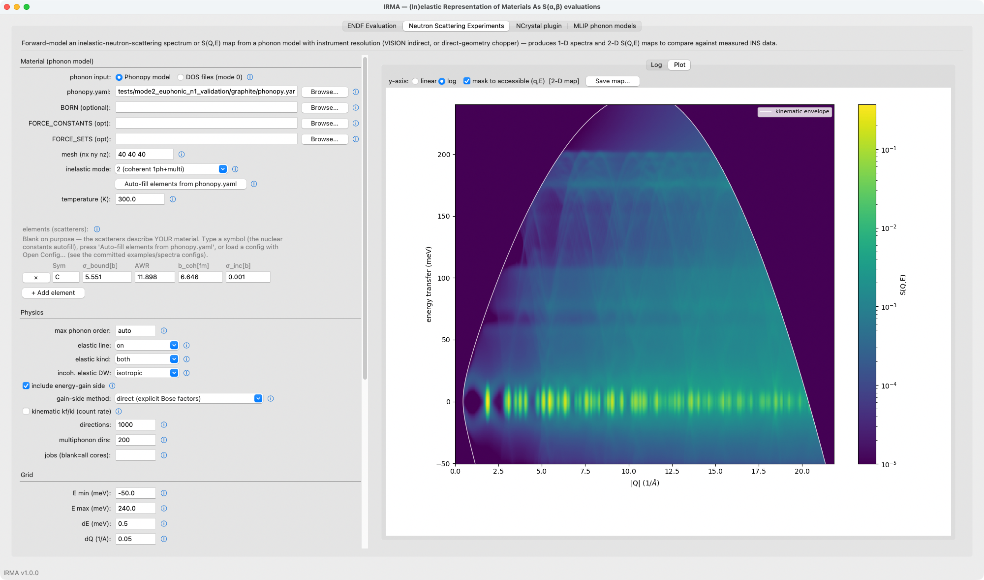
NCrystal plugin tab

This tab writes the per-temperature material data files (.irmapack plus the @CUSTOM_IRMA NCMAT snippet) that the companion transport plugin samples; the data format, the conventions, and the plugin side are documented on the NCrystal data exporter page. The form is the same material block as the other tabs: phonopy.yaml (plus optional BORN / FORCE_CONSTANTS / FORCE_SETS), mesh, temperature, and the scatterer table, which starts as one empty row and autofills its nuclear constants when you type a symbol; then the export settings (material_id, inelastic mode, the powder-average directions and multiphonon dirs, the multiphonon order, the incoherent-elastic Debye-Waller treatment, jobs) and the shared S(α,β) grid section, which is either the converged automatic grid or an explicit alpha/beta pair.

Three actions sit under the output dir:

• Export NCrystal data writes the config to a temporary YAML and runs python -m irma.ncrystal on it out of process, streaming its progress into the Log pane. What the GUI runs is therefore exactly what the command line runs.
• Cancel stops that run and its workers.
• Open Config... reads an exporter config back into the form: one written by this tab, hand-edited afterwards, or the ncrystal.yaml that irma mlip emit generates from a bundle. The file is parsed by the exporter's own loader, so the form accepts nothing the export would reject; a file it refuses reports the reason and leaves the form exactly as it was. Loading replaces the scatterer table with one row per species in the file and selects the grid mode the file implies (explicit when it carries both alpha_grid and beta_grid, automatic otherwise), leaving the other mode's fields at their defaults. Export settings with no control on this form (gain_side, elastic, coherent_partition_mode, site_groups, lat) are carried through unchanged rather than reset, and the Log names the ones that were carried.

---

MLIP phonon models tab

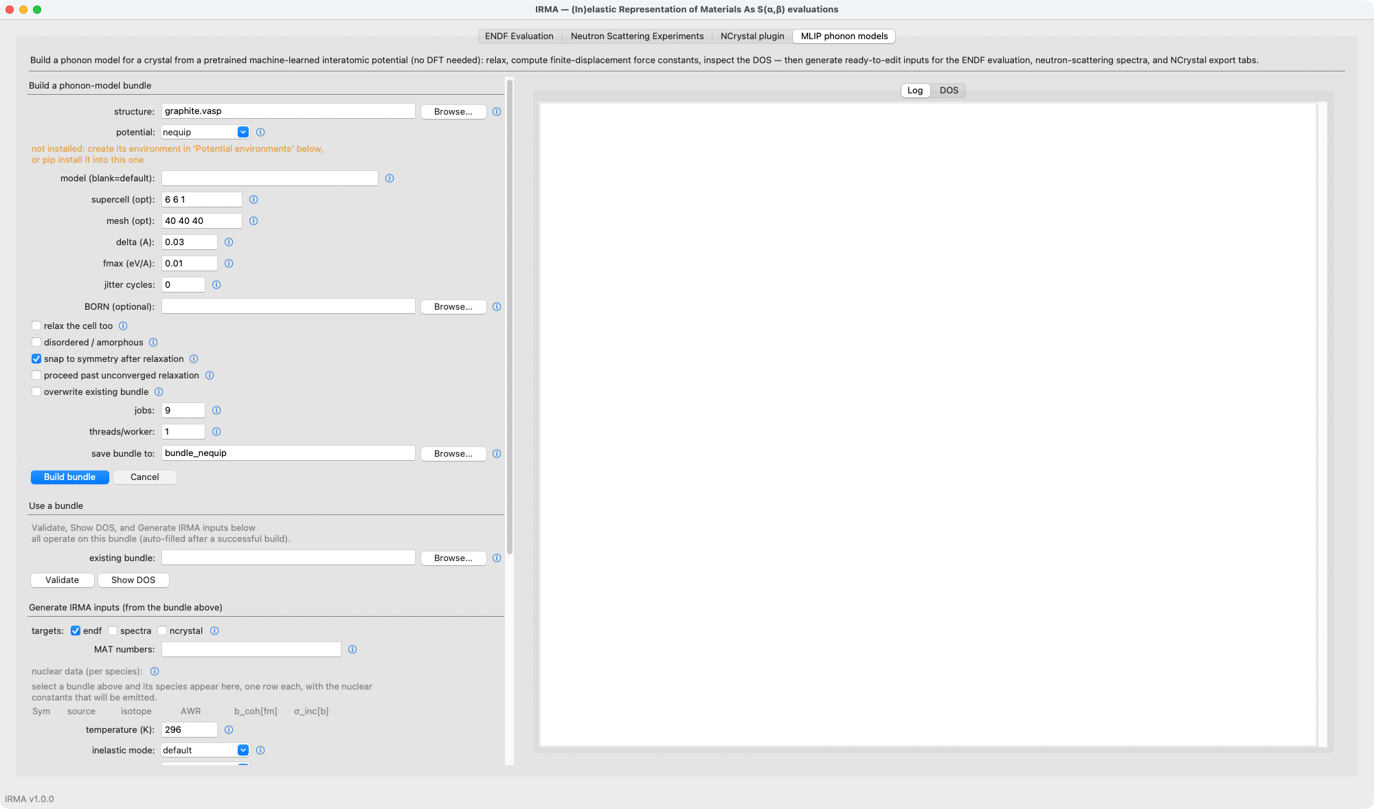
When you have no phonon calculation at all, this tab builds one from a structure file: pick the file and a potential, optionally set the supercell and mesh, and click Build bundle. The form mirrors irma mlip build field for field (every control has the ⓘ help glyph), the Log pane streams the relaxation and force-evaluation progress, and the DOS pane plots the bundle's quick-look DOS after a successful build (or on demand via Show DOS). The sections below the build form operate on a finished bundle, which is auto-filled after a build: Validate re-runs the bundle checks, and Generate IRMA inputs is irma mlip emit: it writes the ENDF input file, spectra YAML, or NCrystal exporter YAML for the selected targets, ready for the other tabs. The Potential environments section creates and removes the per-potential environments that isolate conflicting package pins; it is only needed when a potential's packages are not importable from the running environment. A status line under the build form's potential selector says whether the chosen potential can run right now, and points here when it cannot. The jobs field reveals the matching thread control: a serial-threads field when jobs = 1, a threads-per-worker field when jobs > 1. The Generate IRMA inputs form discloses the same way: only the fields the selected targets read are shown (MAT numbers, inelastic mode and elastic format for endf, material id for ncrystal), and each field's help says which target it feeds. The command line follows the disclosure exactly — a hidden field is neither validated nor passed to the CLI, so a value left over from an earlier selection can neither block the run nor reach it silently.

The scattering constants come from a nuclear data (per species) table in that same form: one row per species in the selected bundle, read from the bundle's own phonopy.yaml as soon as you pick it (a short hint stands in until then). Each row chooses where its constants come from — natural (the default: the natural element, ENDF identity A = 0, natural-abundance constants), isotope (a selector of that element's isotopes; the identity and the constants both switch to it), or custom (b_coh_fm, sigma_inc_b, awr typed in; sigma_bound_b is always derived, never entered). The constants are on screen for every row, read-only unless the row is custom, so you see what will be written before you emit. The table assembles --nuclide and --species for the CLI; a table left alone is all-natural and passes neither flag, which is exactly the emission the CLI performs on its own.

Two things the table handles that the command line can only report after the fact. A species whose tabulated scattering length is an energy-dependent resonance-region value — natural B, Cd, In, Sm, Eu, Gd, or per isotope 6-Li and 10-B but not natural Li or 11-B — opens its own row as custom, with blank boxes and a note saying why; without that, the emit refuses during the cross-target preflight and leaves no files behind to edit. And because an isotope choice changes the constants but not the masses in the phonon calculation, a row warns (never blocks) when the isotope's mass disagrees materially with the mass this bundle's phonopy.yaml carries for that species — selecting 2-H on a bundle built with ordinary hydrogen pairs deuterium constants with hydrogen phonon masses. See MLIP phonon calculations for the potential roster, the conservative-force rule, and the disordered workflow, and MLIP examples for validated end-to-end builds.

---

End-to-end example: graphite, iel=10, inelastic_mode=0

A minimal pass down the form for a crystalline-graphite evaluation:

1. Material: keep iel = 10 and inelastic_mode = 0, then describe the crystal: lattice 2.4612 2.4612 6.7079 90 90 120, and one atom line 6 0 11.898 6.646 0.001 4 0.0 0.0 0.25 0.0 0.0 0.75 0.333333 0.666667 0.25 0.666667 0.333333 0.75. (Both are blank on a fresh form; examples/tsl/graphite_iel10_classic.input is exactly this input file if you would rather import it.)
2. Scattering: enter ZA = 6000, press Fill AWR + sigma_free from ZA (or type AWR = 11.898, sigma_free = 4.739180, the free-atom value; IRMA derives the bound normalization itself), and give the evaluation a MAT number, e.g. 30.
3. Grids: enter 296.0, leave LAT = 1, keep the automatic grid (click Detect from DOS to set Max phonon freq), and Preview Grid Sizes.
4. Phonon: point From phonopy total_dos.dat at your own phonopy total_dos.dat for graphite (two columns: frequency in THz and DOS, as written by phonopy -p mesh.conf; IRMA converts THz→eV on load).
5. Run: choose an output .endf path and click Run Calculation.

For reference, IRMA's mode-0 graphite result with the ENDF/B phonon spectrum overlays the ENDF/B-VIII.1 crystalline-graphite inelastic cross section:

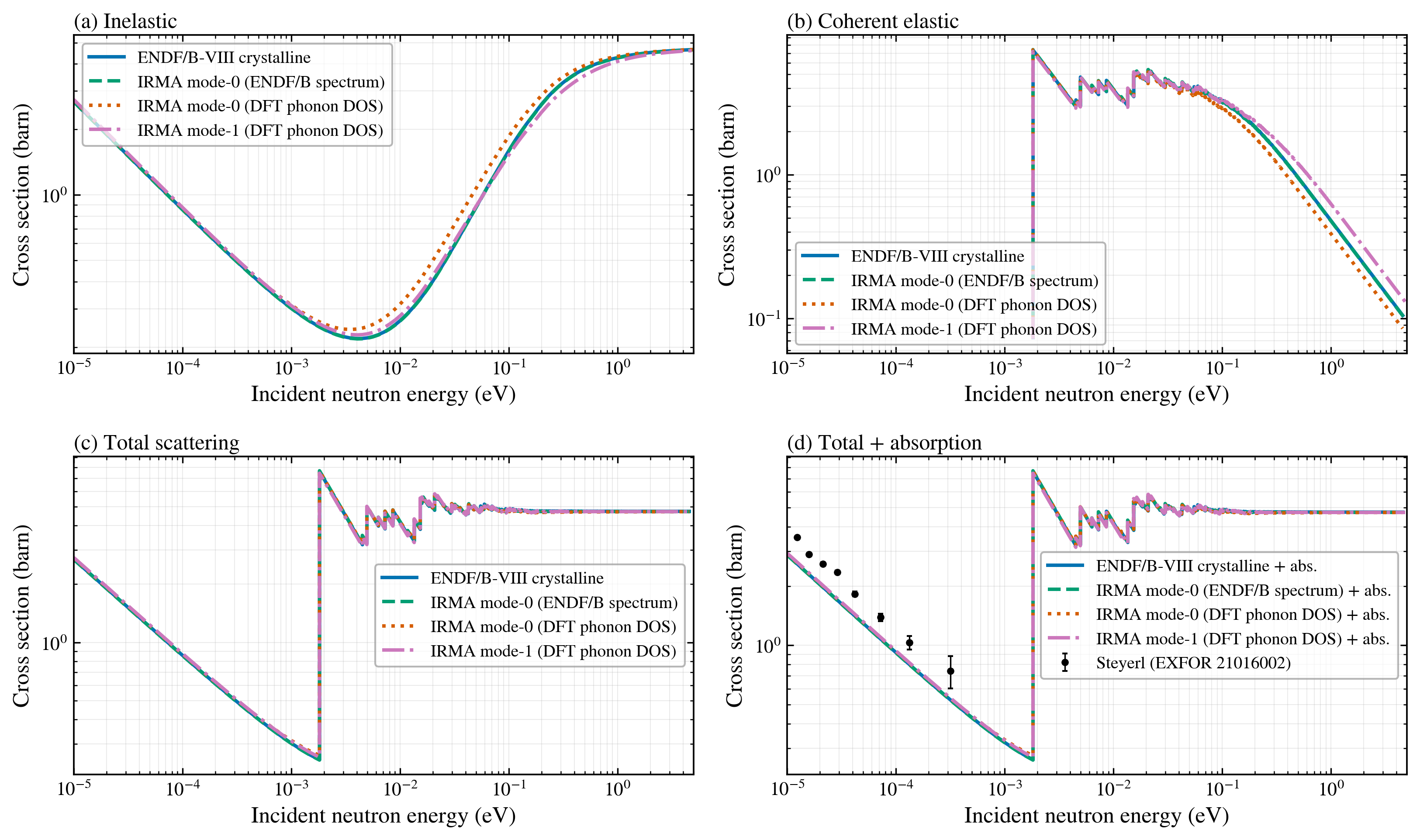
and the linear-in-Q automatic alpha grid recovers the thermal inelastic cross section at a fraction of the column budget of a brute-force reference: