Neutron scattering spectra (irma spectra)

An ENDF tape (a nuclear data file; "tape" is the historical name) tells a transport code such as MCNP or OpenMC how a material scatters; it does not tell you what your instrument will measure. IRMA's forward model closes that gap. It takes the same phonon physics the ENDF side evaluates and turns it into the quantities an instrument records, an instrument-resolved 1-D inelastic neutron scattering (INS) spectrum or a dense 2-D S(Q,E) powder map, with no ENDF tape involved. The calculation computes a powder S(Q,E), projects it onto the instrument's kinematic locus (the path through (Q,E) the geometry can reach: fixed final energy for indirect geometry, fixed incident energy for direct), convolves it with an energy-resolution model, and adds an elastic line built from the same Debye-Waller factors as the inelastic part. Use it to preview an experiment before beam time, to compare a phonon calculation against measured data, or to sanity-check an evaluation by looking at it the way a beamline would.

The physics level is the same inelastic_mode as on the ENDF side (see Scattering modes): mode 0 builds S(Q,E) straight from a phonon density of states (DOS), with no eigenvectors (see DOS-based spectra (mode 0) for that whole workflow), while modes 1 and 2 run the noncubic engine (the incoherent approximation, or the exact coherent one-phonon term) on a phonopy.yaml plus force constants (Preparing a phonopy calculation covers producing one). The model covers VISION, generic indirect, and direct (chopper) geometries, with an automatic chopper resolution model validated against PyChop. Install the extra first: pip install -e ".[spectra]" (plus [phonopy] for modes 1/2).

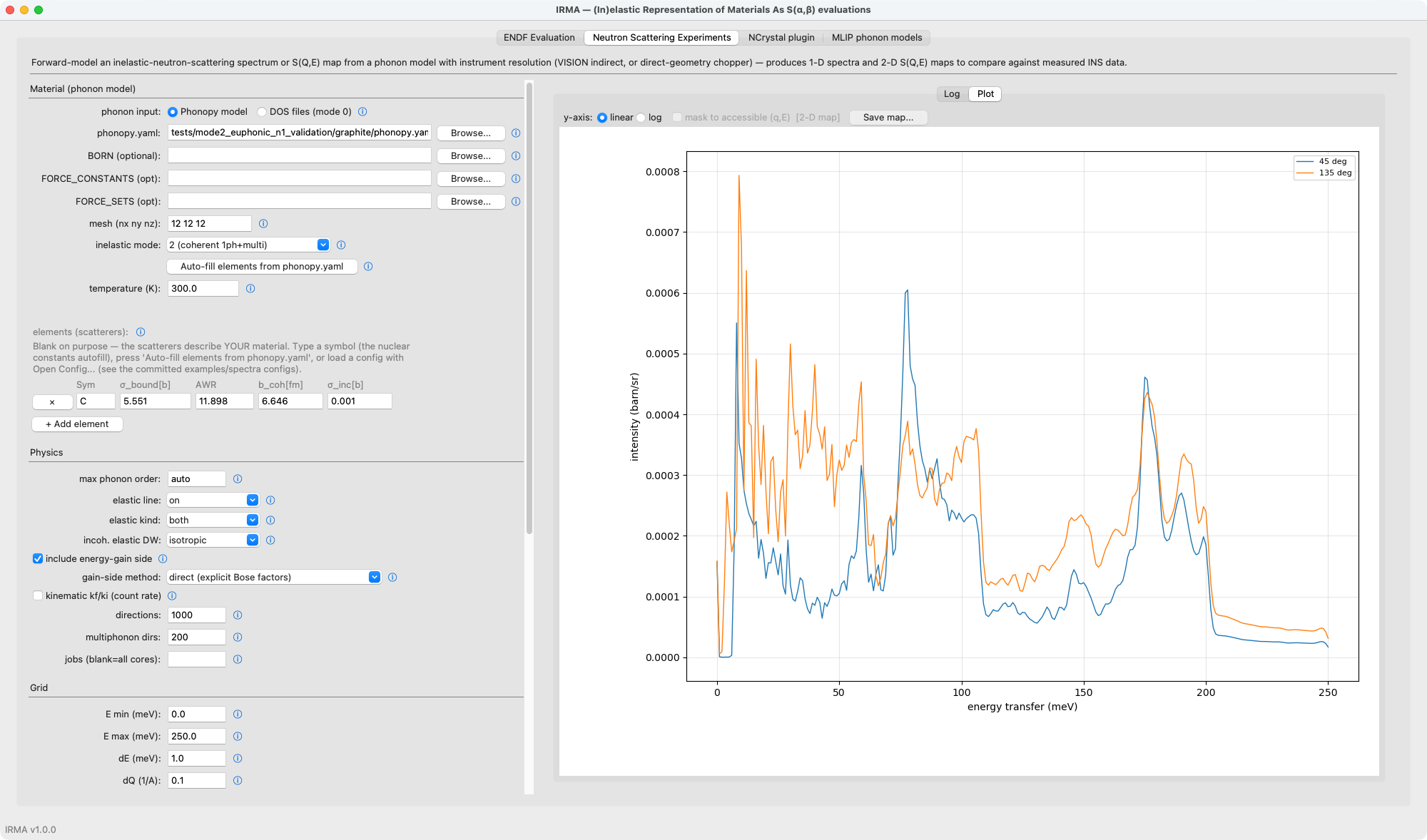
An end-to-end example: graphite, mode 2, two instruments

The committed examples are the fastest orientation. From examples/spectra/ (the configs use paths relative to that directory), the highest-fidelity 1-D spectrum (exact coherent one-phonon, anisotropic Debye-Waller, VISION resolution) is one command:

cd examples/spectra
python -m irma spectra run graphite_mode2_vision.yaml -o graphite_vision.csv

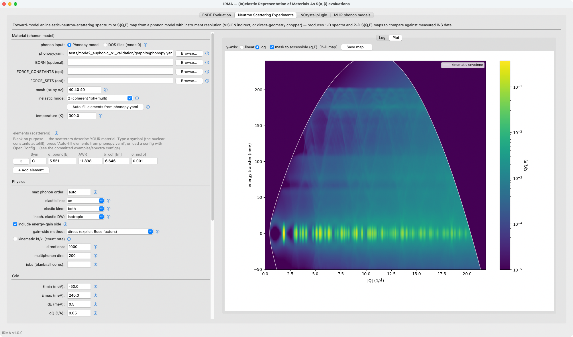
and the same phonon calculation becomes a direct-geometry ARCS S(Q,E) map, with the chopper resolution computed automatically and the map masked to the detector coverage:

python -m irma spectra map graphite_arcs_map.yaml -o graphite_arcs.npz

These are the two product shapes (per-bank energy spectra and the 2-D map), shown here as the GUI's Plot pane renders them (the CLI writes the same data to CSV/npz):

The rest of this page is the reference for driving the model: the CLI subcommands, every flag, and the config-file schema. The GUI face of the same model is the Neutron Scattering Experiments tab, covered in the GUI guide.

Two ways to drive it

Two entry points drive the model, and they share exactly one compute path:

• Flag form: irma spectra vision|indirect|direct … builds a config from command-line flags. A convenience layer for quick runs.
• Config form: irma spectra run <config> -o out.csv (or map) loads a SpectraConfig file (YAML / TOML / JSON). This form is reproducible, and the GUI writes these files.

All temperatures default to 296 K; override with --temperature (flag form) or material.temperature_K (config form).

CLI subcommands

vision: VISION preset (indirect)

irma spectra vision \
    --phonopy-yaml graphite/phonopy.yaml --mesh 40 40 40 \
    --inelastic-mode 2 \
    --scatterer C,5.551,11.898 \
    -o graphite_vision.csv

The VISION preset fills in its own Ef = 3.5 meV, its 45°/135° banks, and the published resolution polynomial; override Ef with --ef.

indirect: generic fixed-final-energy geometry

irma spectra indirect --ef 3.5 --angles 45,90,135 \
    --phonopy-yaml model.yaml --inelastic-mode 2 \
    --scatterer C,5.551,11.898 -o spec.csv

--angles accepts a comma list (45,90,135) or an inclusive start:stop:step range (30:150:15).

direct: generic fixed-incident-energy geometry

irma spectra direct --ei 250 --e-max 245 --angles 5:140:5 \
    --resolution-model chopper --chopper-instrument ARCS \
    --chopper-package ARCS-700-1.5-AST --chopper-frequency 600 \
    --phonopy-yaml model.yaml --inelastic-mode 2 \
    --scatterer C,5.551,11.898 -o arcs.csv

Direct geometry requires --e-max strictly below Ei (a neutron cannot lose its full incident energy and still reach the detector). Since the --e-max default is 250 meV, --ei 250 needs an explicit --e-max or a higher Ei. --resolution-model chopper auto-computes the energy resolution for any of the eight supported direct-geometry instruments (ARCS, SEQUOIA, MAPS, MARI, MERLIN, HYSPEC, CNCS, LET). --kinematic-factor multiplies by kf/ki for a count-rate spectrum.

run: execute a config file

irma spectra run material.yaml -o spec.csv --set material.temperature_K=500

--set a.b.c=value applies dotted overrides on top of the file (repeatable).

map: dense 2-D S(Q,E) powder map

irma spectra map material.yaml --q-min 0.0 --q-max 12 --dq-map 0.05 \
    --angle-range 5 140 --mask -o map.npz

The map runs for any geometry; the kinematics follow the config's instrument.geometry. --angle-range MIN MAX attaches the instrument's kinematic envelope, and --mask blanks S(Q,E) outside the accessible "arch". Output is .npz (the default) or long-form .csv.

With physics.elastic: true (the default) the map carries the same elastic model as the 1-D spectra: the per-Q elastic cross section appears as a ridge at E = 0 (the Bragg peaks plus the incoherent Debye-Waller line, smeared over the map's --dq-map Q bin) and is broadened by the energy-resolution model like every other feature. A subtlety for absolute-intensity comparisons only: the two products deliberately differ in how they normalize the elastic line when the energy axis starts at 0 (e_min = 0, the default). The 1-D spectra renormalize the visible half-peak so that its integral equals the full per-Q elastic area; the map instead deposits area/dE in the boundary bin, which retains only half the area under trapezoidal integration (the run prints a NOTE when this applies). For absolute-intensity comparisons between the map and the 1-D spectra, use e_min < 0 so the whole line is on-axis and the two conventions agree.

Common flags (all geometries)

Flag	Meaning	Default
--inelastic-mode {0,1,2}	0 = DOS + isotropic Debye-Waller; 1 = incoherent approximation; 2 = exact coherent 1-phonon + incoherent multiphonon	2
--scatterer	SYMBOL,sigma_bound_b,awr[,b_coh_fm[,sigma_inc_b]]: bound cross section [b], atomic weight ratio (mass over neutron mass), coherent scattering length [fm], incoherent cross section [b]; IRMA's built-in nuclear-data table supplies all four for any element (the GUI and irma mlip emit fill them automatically). Mode-0 key=value tokens (dos=, unit=, mult=, pos=) append. Repeatable.	—
--mesh NX NY NZ	phonon q-mesh	40 40 40
--temperature	sample temperature (K)	296
--de / --e-min / --e-max	energy grid step / start / end (meV); negative e-min adds the energy-gain side	0.5 / 0 / 250
--dq	S(Q,E) Q-support spacing (1/Å)	0.05
--max-phonon-order	multiphonon order; auto sizes to convergence in every mode (mode 0 derives it from the DOS's Debye-Waller integral)	auto
--directions / --mp-directions	modes 1/2 coherent / multiphonon powder-average directions	10000 / 1000
--elastic {on,off} / --elastic-kind {both,coherent,incoherent}	elastic line	on / both
--gain-side {direct,detailed_balance}	energy-gain (E<0) evaluation: explicit Bose factors vs detailed-balance mirror	direct
--resolution-shape {gaussian,lorentzian}	line shape	gaussian
--jobs	worker processes	all cores
-o, --output	output .csv (default) / .npz / .json	required

Config file reference (SpectraConfig)

A config file is a mapping of four sections: material, physics, grid, instrument. All keys below are optional except material.scatterers (and material.phonopy_yaml for modes 1/2; Preparing a phonopy calculation covers how to make one from your own force calculation). The GUI writes these files, or you can write them by hand in YAML, TOML, or JSON.

material

Key	Type	Default	Meaning
phonopy_yaml	str	—	phonopy calculation; required for modes 1/2 and mode-0 dos_source: phonopy
force_constants / force_sets / born	str	discovered	explicit FC / FORCE_SETS / BORN (NAC) files
mesh	[nx,ny,nz]	[40,40,40]	phonon q-mesh
temperature_K	float	296	sample temperature
scatterers	list	—	per-species scattering data (see below)
lattice	[a,b,c,α,β,γ]	—	mode-0 only, unit cell (Å, deg) for the coherent-elastic Bragg peaks

Each scatterer entry: symbol, sigma_bound_b, awr, optional b_coh_fm, sigma_inc_b, and mode-0 fields dos_file, dos_unit (meV|eV|cm-1|THz), multiplicity, positions (fractional [x,y,z] sites for the elastic Bragg peaks).

physics

Key	Default	Meaning
inelastic_mode	2	0 DOS / 1 incoherent-approx / 2 coherent 1-phonon + incoherent multiphonon (2, the validated mode, is the default)
dos_source	file	mode-0 DOS origin: per-scatterer dos= files or phonopy
max_phonon_order	auto	int ≥ 1 or auto
n_directions / multiphonon_directions	10000 / 1000	powder-average directions (modes 1/2)
jobs	null (all cores)	worker processes
elastic / elastic_kind	true / both	elastic line on/off and channel (both/coherent/incoherent)
elastic_from_tape	—	build the elastic line from an ENDF tape's elastic section (MF7/MT2) instead of from the phonon calculation
incoherent_elastic_mode	isotropic	Debye-Waller treatment of the incoherent elastic line: isotropic (one scalar Debye-Waller parameter per species, the trace/3 W′ the ENDF convention stores) or directional (powder-averaged anisotropic ⟨exp(-Q² û·U·û)⟩ per atom; modes 1/2 only; needs the engine's displacement tensors). Same option name as the NCrystal export.
include_energy_gain	true	add the energy-gain (E<0) side
gain_side	direct	energy-gain (E<0) evaluation. direct computes the gain side with explicit Bose occupation factors in every mode (the energy-loss output is unchanged); detailed_balance mirrors the loss side instead. The two agree to sub-bin level, with direct the more accurate: it uses each line's true energy, not the loss bin center
kinematic_kf_ki	false	multiply by kf/ki (count-rate spectrum)

grid

Key	Default	Meaning
e_min_meV / e_max_meV / de_meV	0 / 250 / 0.5	energy-transfer grid (negative e_min includes energy gain)
dq_max_invA	0.05	S(Q,E) Q-support spacing
q_max_invA	—	2-D map Q-axis maximum (1-D runs derive Q from the instrument)

instrument

Key	Default	Meaning
geometry	vision	vision / indirect / direct
e_fixed_meV	3.5	Ef (vision/indirect) or Ei (direct)
angles_deg	preset	detector angles (deg)
q_cuts	—	constant-|Q| cuts (1/Å); honored whenever supplied, alongside the angle/bank spectra
bank_halfwidth_deg	5	detector-bank angular half-width
sigma_coeffs	preset	resolution width polynomial σ(E) = c0 + c1·
resolution_shape / resolution_model	gaussian / poly	line shape; poly or chopper
chopper_spec	—	{instrument, package, frequency} for resolution_model: chopper
combine	mean	combine detector banks by mean or sum
output_mode / cut_by	cuts / angles	cuts (1-D spectra) or map (dense 2-D S(Q,E), any geometry); cut_by (direct geometry only): angles (bank spectra, plus any q_cuts) or q (constant-Q cuts only)
cut_dq_invA	—	constant-Q cut band width (None → thin slice)
map_coverage_deg / map_mask	— / true	2-D map kinematic envelope band + masking
export_components	false	also write the inelastic + elastic breakdown (else total only)

The physics.inelastic_mode choice decides what the model needs from you. Mode 0 builds S(Q,E) straight from a per-species phonon DOS, with no eigenvectors; it is fast and well suited to incoherent and hydrogen-rich materials, and DOS-based spectra (mode 0) covers that whole workflow. Modes 1 and 2 use the phonopy eigenvectors (mode 2's exact one-phonon term is built from them).

Which chopper was in the beam? (finding chopper_spec)

resolution_model: chopper needs the Fermi chopper package and frequency that were actually in the beam for the run you are modeling. It is important to note that these must come from the data, not from the nominal beam-time request: the two can differ, and the choice matters, since a 0.5 mm versus a 1.5 mm slit package changes the elastic width by roughly 2×. On ARCS (SNS), the in-beam Fermi package is recorded in the raw NeXus file as the DAS log BL18:Chop:InUse:ChopperId, and the Fermi speed is in the chopper-frequency log; the reduced NXSPE or processed file usually also carries the incident energy and chopper settings in its metadata. Other direct-geometry instruments expose the same information under their own log names. Look up the in-beam chopper id and speed for the specific run.

What the forward model captures, and what it does not

The forward model computes a single-scattering, powder-averaged S(Q,E) and convolves it with an energy-width resolution model: it supplies the calculated single-scattering counterpart of a measured spectrum, and it models nothing else about the measurement. That scope keeps it fast and makes its output a clean expression of the phonon calculation, but it also means several real measurement effects are deliberately absent. Read any comparison against measured data with them in mind.

Single scattering only. IRMA scatters each neutron once. A real sample of any appreciable thickness also multiply-scatters, and multiple scattering adds a broad inelastic background that piles up under and beside the phonon features. The visible symptom is the elastic-to-inelastic balance: the single-scattering calculation keeps too much weight in the elastic line relative to the inelastic continuum, and the gap grows with incident energy and sample thickness. For a millimeter-thick graphite plate on a direct-geometry chopper spectrometer, the single-scattering elastic/inelastic area ratio runs roughly 1.5–2.5× high versus the measurement (growing with Ei), while the phonon peak positions and the relative one-phonon intensities stay correct. Treat absolute inelastic intensities and the elastic/inelastic ratio as model bounds, not predictions.

Resolution is a Gaussian width, not a full lineshape. The chopper model (resolution_model: chopper) reproduces PyChop's energy-dependent width (the full width at half maximum, FWHM) to ~1%, and that width is applied as a symmetric Gaussian. PyChop itself emits only a variance, so there is no lineshape to borrow. The true elastic line is mildly asymmetric: the moderator emission pulse leaves a small tail on the energy-gain side, strongest at low incident energy (half-width asymmetry ≈ 1.2–1.5 at Ei ≈ 30 meV) and fading to near-symmetric by a few hundred meV. The Gaussian is a good approximation everywhere except the low-Ei wings; it does not model the moderator-pulse, detector-depth, or sample-size contributions to the line shape, only their contribution to the width, through the chopper model.

No sample or instrument geometry. There is no self-shielding or absorption, no sample-can or sample-environment scattering, no detector efficiency or angular-coverage gaps, and no detector-binning kinematics. The 2-D map is an idealized powder S(Q,E) on the instrument's kinematic locus.

When you need the full instrument: McStas and McVINE

For anything that depends on the effects above (multiple scattering, the real moderator-pulse lineshape, detector geometry and efficiency, sample self-shielding, or absolute intensities), model the instrument with a Monte Carlo package such as McStas or McVINE, using IRMA (or an NCrystal or ENDF kernel built from the same physics) as the sample scattering kernel. IRMA's forward model is the right tool for previewing features and for comparing a phonon calculation to data on an equal footing; a Monte Carlo instrument model is the right tool for reproducing a measured spectrum in full. The graphite validation in this project pairs the two exactly this way: IRMA for the phonon physics, a McStas virtual experiment for the instrument and multiple scattering.

One caveat when reading such an overlay: the Monte Carlo sample kernel and IRMA may not use the same inelastic physics. The McStas/NCrystal graphite kernel used here, for example, evaluates the inelastic scattering in the incoherent approximation, whereas IRMA mode 2 computes the coherent one-phonon term, so where the two inelastic continua differ, part of the difference is the scattering model itself, not multiple scattering alone.