Automatic grids

IRMA tabulates the thermal scattering law \(S(\alpha,\beta)\) on a grid of dimensionless momentum transfer \(\alpha\) and energy transfer \(\beta\). Everything downstream is computed from that table: the inelastic cross section and the secondary energy distributions that THERMR (the NJOY module that processes the tape) reconstructs, and the size of the ENDF tape itself.

A grid that is too coarse in the wrong place silently under-integrates the cross section; a grid that is too fine everywhere produces enormous tapes for no accuracy gain. This page explains the automatic \(\beta\) and \(\alpha\) grids IRMA builds for you, the physics behind their shapes, the validated accuracy you can expect, and when to override them by hand to match a reference evaluation.

Automatic grids are built in the GUI (the ENDF form's Grids part) or through the irma.core.grids functions from Python. The GUI writes the resulting explicit Cards 7–9 into the input file; there is no auto-grid flag in the card format.

Why the grid shape matters

The tabulated \(S(\alpha,\beta)\) is the only thing the cross-section integrators see. The thermal-energy inelastic cross section is dominated by a narrow band of small \(\alpha\) (the upscatter windows: the region where thermal neutrons gain energy from the lattice, roughly \(\alpha \sim 0.01\text{–}0.3\), equivalently momentum transfer \(Q \sim 1\text{–}6\ \text{Å}^{-1}\)), while the \(\beta\) direction must resolve the phonon spectrum's peaks and van Hove singularities (the kinks and spikes a phonon DOS has where a branch is flat). The two axes therefore need different spacing, and IRMA's automatic grids concentrate points where the integrands vary rather than spreading them uniformly.

The beta grid: three regions

generate_beta_grid builds the energy-transfer axis in three contiguous regions, each with its own GUI control. The grid always starts at \(\beta = 0\).

Region	Spacing	GUI parameter	What it captures
Lower tail	Logarithmic, from \(\beta_\min = 10^{-9}\ \text{eV}/kT\) up to the phonon region	Beta N lower (log)	Thermal quasi-elastic scattering very near \(\beta = 0\), where \(S(\alpha,\beta)\) varies rapidly
Phonon region	Linear, spacing \(\text{freq\_max}/\text{N\,phonon}\) over \((0, \text{freq\_max})\)	Beta N phonon (linear)	The phonon spectrum itself: peaks and singularities resolved uniformly
Upper tail	Logarithmic for log-lin (iint=0) input files; step-capped out to a few ridge widths past the back-scatter alpha for lin-lin (iint=1) input files (see the lin-lin upper tail)	Beta N upper (log) and Beta max	Multiphonon contributions and the smooth exponential high-energy tail

For inelastic_mode 1/2 the one-phonon term is zero below the lowest mesh-mode energy of the phonopy q-mesh (the run prints it), however fine the lower tail is.

The linear phonon region runs up to the maximum phonon frequency freq_max, which you can enter directly or auto-detect from a DOS file or phonopy.yaml in the GUI. The upper tail extends to Beta max (default 5 eV). The 5 eV default suits most solid moderators, but hydrogen's large recoil pushes significant scattering well past 5 eV; give hydrogen 10 eV or more so the tabulated \(S(\alpha,\beta)\) is not truncated.

The alpha grid: linear in momentum transfer

The \(\alpha\) axis (generate_alpha_grid) is linear in momentum transfer \(Q\), which makes \(\alpha\) quadratic in \(Q\). Points are placed at \(Q = \text{dQ}, 2\,\text{dQ}, \dots\) up to a cutoff \(Q_\text{cut}\), after which a logarithmic tail runs out to the maximum \(Q\) that matches the \(\beta\) grid's kinematic reach, \(\alpha_\max = 4\beta_\max/A\) (\(A\) is the scatterer's mass ratio to the neutron). Each grid \(Q\) maps to \(\alpha\) through

\[ \alpha = Q^2 \,\frac{\hbar^2/2m}{A\,kT}. \]

The map from \(Q\) to \(\alpha\) contains \(kT\), so the grid is built at one reference temperature: 293.6 K for lat=1 (the \(Q\) grid is then the same at every deck temperature) or the first deck temperature for lat=0.

Why not mirror the beta grid?

Mirroring the \(\beta\) grid through the recoil relation \(\alpha = 4\beta/A\) would copy \(\beta\)'s linear-in-energy layout onto \(\alpha\). But the thermal cross section is governed by \(S(\alpha,\beta)\) in the upscatter windows at small \(\alpha\) (\(Q \sim 1\text{–}6\ \text{Å}^{-1}\)), and there a constant-\(\Delta\alpha\) grid is several times too coarse compared with the quadratic-in-\(Q\) spacing the physics asks for. Putting points uniformly in \(Q\) concentrates resolution exactly where the integrand is sharp.

Validated accuracy

On graphite at 296 K (all five grids scored with the same thermr_mimic inelastic cross section on the same incident-energy nodes, below ~25 meV; thermr_mimic is the validation record's own implementation of THERMR's cross-section integration, not shipped with IRMA and described on the NJOY interoperability page), the default grid and every finer grid agree; only a deliberately coarse grid under-resolves the thermal window:

Resolution class	Thermal inelastic XS vs the dQ = 0.01 reference
dQ = 0.25 (deliberately coarse)	12% low at the 5 meV minimum, up to 29% off near 8.3 meV
uniform dQ = 0.05 (2000 columns)	−0.33% on the 0.01–25 meV integral, 1.2% rms pointwise
dQ = 0.01 (finer)	reference; halving dQ again moves the integral by −0.001% (0.27% maximum)
automatic grid, default (399 columns)	same agreement as dQ = 0.05, at a fifth of the columns

The default dq_ang_inv = 0.05 is already converged. The largest local difference is 4.3% (at 2.12 meV), among the narrow unbroadened coherent features in the thermal window around the inelastic cross-section minimum, where the cross section is only about 0.25 b (a few percent of the total). The compact automatic grid reaches the same agreement with 399 alpha columns against 2000 for uniform dQ = 0.05 (5.72 MB of tape against 27.22 MB), which is why it is the shipped default.

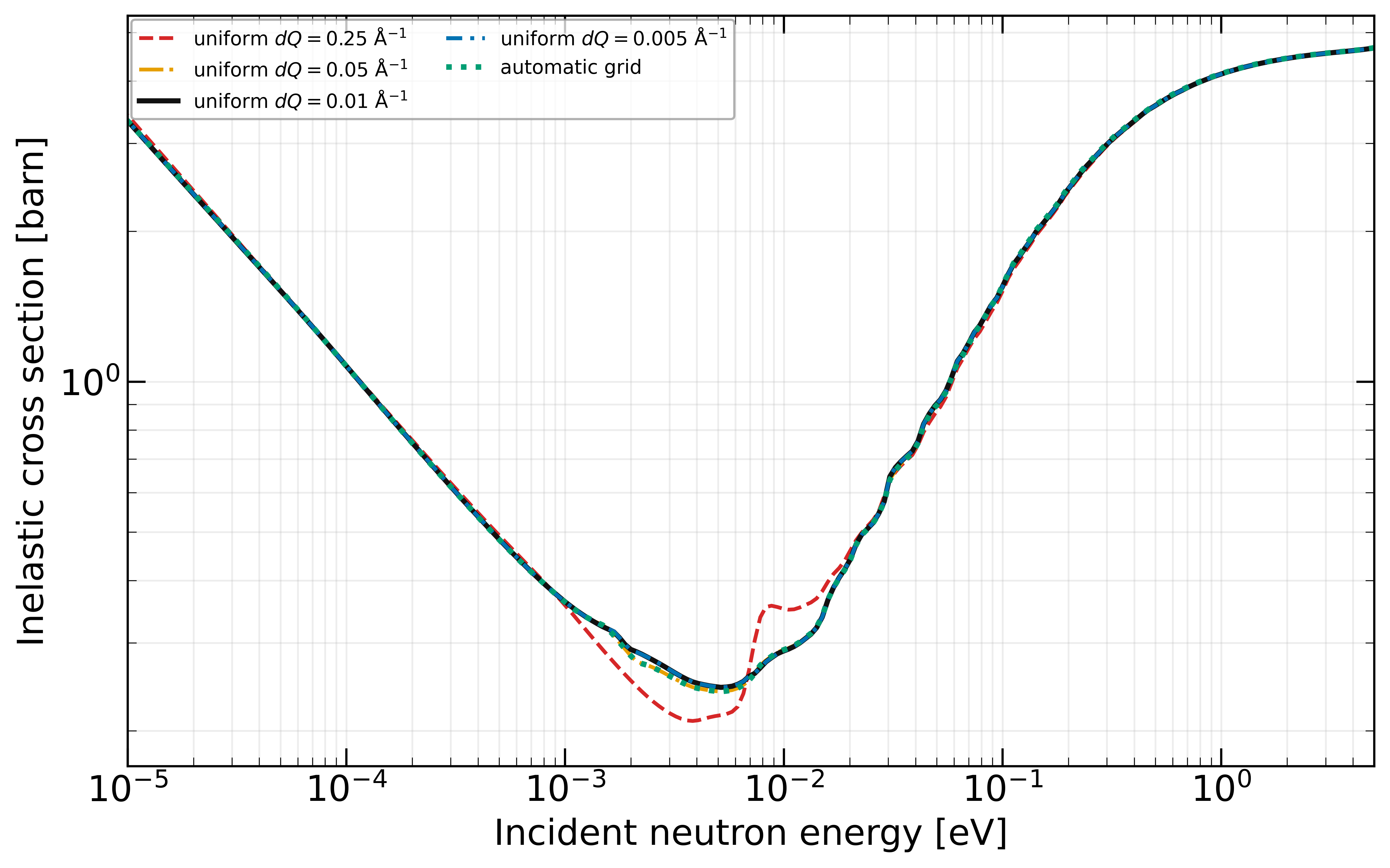The compact automatic grid (green dotted) reproduces the converged dQ = 0.05, dQ = 0.01, and dQ = 0.005 cross sections across the whole range; only the deliberately coarse dQ = 0.25 grid under-resolves the thermal window, and no grid overshoots the free-atom limit at high energy. All five grids scored with the same thermr_mimic implementation on the same incident-energy nodes.

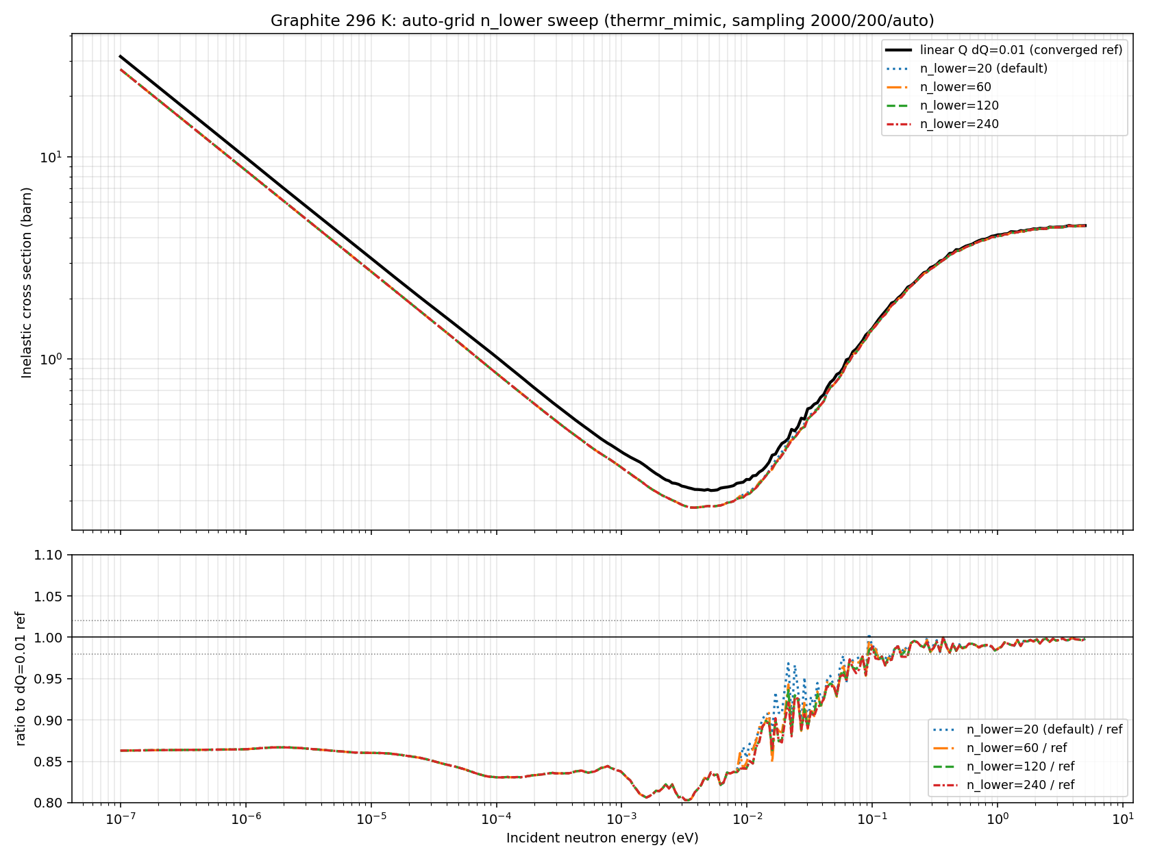Sweeping the number of low-beta logarithmic points: the thermal peak stabilizes once the lower tail is adequately resolved.

Defaults

Parameter	GUI label	Default	Meaning
n_lower	Beta N lower (log)	15	Low-\(\beta\) logarithmic points (GUI default; the generate_beta_grid function default is 50)
n_phonon	Beta N phonon (linear)	300	Linear subdivisions of the phonon region \((0, \text{freq\_max})\)
n_upper	Beta N upper (log)	80	High-\(\beta\) tail density (GUI default; the generate_beta_grid function default is 20 for log-lin grids and 80 for lin-lin). On a lin-lin (iint=1) grid the tail gains extra step-capped points below the recoil ridge (the band \(\alpha \approx \beta/A\) where free-recoil scattering peaks), so the final tail count exceeds n_upper (see below)
beta_max_eV	Beta max	5.0 eV	Upper bound of the \(\beta\) grid
dq_ang_inv	Alpha dQ	0.05 Å⁻¹	\(Q\) spacing of the linear \(\alpha\) segment
q_cut_ang_inv	Alpha Q cut	12.0 Å⁻¹	End of the linear segment (set by neutron kinematics, not the material)
n_log	Alpha N log	160	Logarithmic \(\alpha\) points from \(Q_\text{cut}\) to \(Q_\max\)

The \(\alpha\) and \(\beta\) grids are independent: nalpha is decoupled from nbeta, so you can refine one axis without inflating the other.

The Alpha Q cut is set by neutron kinematics, not by the material's phonon cutoff: the linear segment must cover the thermal upscatter windows. The default 12.0 Å⁻¹ rarely needs changing.

The upper tail on lin-lin (INT=2) grids

The two flag names map one-to-one: the input file's Card 4 iint=0 writes ENDF interpolation law INT=4 (log-lin), and iint=1 writes INT=2 (lin-lin).

A purely logarithmic tail lets the step grow without bound: \(\Delta\beta \approx 30\) near the default \(\beta_\max\) for the coarse n_upper=20 tail. Log-lin (INT=4) interpolation tolerates that, because INT=4 reproduces the \(\exp(-\beta/2)\) detailed-balance tail exactly on any grid. Lin-lin (INT=2) interpolation instead connects the tabulated points with straight lines, and across a step that wide the straight segments lie far above the decaying exponential between the points, so the reconstructed cross section overshoots the free-atom cross section by more than 100% at high incident energy. The grid builder therefore keys the tail on the input file's Card 4 iint flag (generate_beta_grid(..., iint=...); the GUI, irma mlip emit, and the NCrystal pack exporter all build their \(\beta\) grids through it):

• iint=0 (log-lin): the tail is purely logarithmic with n_upper points.
• iint=1 (lin-lin): the tail is step-capped up to a limit set by the recoil ridge, then logarithmic:
  • Step cap. The logarithmic step is capped at \(\Delta\beta = 0.5\) (DELTA_BETA_MAX_LINLIN; the exact midpoint overshoot of \(\exp(-\beta/2)\) at that step is \(\cosh(0.125) - 1 \approx 0.78\%\)) from the end of the phonon region up to linlin_fine_beta_limit.
  • Ridge margin. That limit is the back-scatter \(\alpha\) at the highest incident energy (the largest \(\alpha\) the \(\beta\) grid can reach, \(\alpha_\max = 4\beta_\max/A\)), plus RIDGE_MARGIN_SIGMAS widths of the down-scattering kernel there. Above the limit \(S(\alpha,\beta)\) is the off-ridge tail and the coarse log spacing resumes.
  • Width bound. THERMR integrates the stored symmetric law times \(e^{+\beta/2}\), which in the short-collision-time form is a Gaussian in \(\beta\) centered at \(\alpha\) with standard deviation \(\sqrt{2\alpha T_\text{eff}/T}\). The generator knows only freq_max, so it uses the bound \(T_\text{eff}/T \le (x/2)\coth(x/2)\) with \(x = E_\max/kT\) (effective_temperature_bound_ratio), which no spectrum ending at \(E_\max\) exceeds (a Debye spectrum with that cutoff sits 10 to 13% below it). The width grows with the evaluation temperature, so the limit is taken at the hottest temperature in the deck.
  • Low-temperature scaling. The cap is a physical \(\beta\) step. A lat=1 grid is written in 0.0253 eV units, so for a deck whose lowest temperature is below 293.6 K the stored cap is scaled by \(T_\text{lowest}/293.6\,\text{K}\) (evaluation_temperatures_K); otherwise a 0.5 stored step at 77 K would be a 1.9 physical step with an 11.6% midpoint error.
  • Reporting. The tail has more than n_upper points and is not logarithmic; the deck emitters, the GUI grid preview, and the NCrystal exporter print one line with the point count, the energy the grid reaches and the tail type. Where the capped and logarithmic parts meet, a node that would print as a duplicate of its neighbor at the deck's six decimals is dropped, so the written grid is strictly increasing.

Ending the fine step at \(\alpha_\max\) is not enough: on graphite at 296 K the cells just above it are still populated at the highest incident energies, and lin-lin interpolation across the coarse cells there raised the total cross section between 2 eV and the requested energy by 0.8% for a 5 eV grid and by 2.6% for a 10 eV grid (patched NJOY THERMR honoring INT=2, incoherent approximation, values read from the processed PENDF at the requested energy), while the same tape processed log-lin stayed flat. The margin was calibrated on those runs; the rise from 2 eV to the requested energy is

RIDGE_MARGIN_SIGMAS	5 eV grid	10 eV grid
1	0.13% (501 points)	0.19% (649 points)
1.5	0.09% (521)	0.11% (680)
2	0.09% (541)	0.10% (710)

so 2 widths reach the converged value at both extents. What remains is the cost of the 0.5 step itself: halving the step to 0.25 lowers the whole lin-lin curve by about 0.3% (the step's own bias, consistent with the 0.78% midpoint overshoot) and leaves a rise of 0.02% (5 eV) and 0.03% (10 eV) from 2 eV to the requested energy, at 747 and 1089 \(\beta\) points. The margin costs points: a lin-lin graphite grid to 5 eV has 541 \(\beta\) points against 395 for log-lin, and one to 10 eV has 710.

The GUI defaults n_upper to 80; the generate_beta_grid log-lin default is 20.

Manual grids: matching a reference evaluation

When you need IRMA's grid to match an existing evaluation column-for-column (for a direct tape comparison, or to reproduce a published LEAPR input file), supply the grids explicitly on Cards 7–9 instead of letting IRMA build them. The input file format is NJOY free-format:

nalpha nbeta lat /        $ Card 7: grid sizes; lat=1 = grids at the 0.0253 eV reference temperature
a1 a2 a3 ... /            $ Card 8: nalpha alpha values, strictly increasing, all > 0 (may span lines)
b1 b2 b3 ... /            $ Card 9: nbeta  beta  values, strictly increasing, from >= 0

Both lists must be strictly increasing; the \(\alpha\) values must be positive and the \(\beta\) values may start at zero. With lat=1 the grids are interpreted as being given at the 0.0253 eV reference temperature, exactly as in LEAPR.

No grid choice, manual or automatic, protects a tape from one defect in stock NJOY2016 THERMR: a coherent mode-2 table (inelastic_mode=2, the exact coherent one-phonon treatment) can trigger the cliq liquid-extrapolation guard regardless of the grid spacing, because the failure follows the shape of the tabulated \(S(\alpha,\beta)\), not whether the \(\beta\) grid is uniform. See NJOY interoperability for the symptom and the one-line patch; mode-0/1 tapes and most materials are unaffected.

Grid size also drives file size directly: ENDF tapes carry roughly 6-significant-figure values, so a 2000×5001 grid is on the order of 270 MB. Refine only the axis and region that needs it.