Tutorial: an ENDF evaluation from a phonopy calculation

This tutorial produces a production-quality thermal scattering evaluation for graphite: one committed input file in, one ENDF-6 tape out, in about a minute on a laptop. (A tape is an ENDF output file, the historical name, and S(α,β) is the thermal scattering law in the dimensionless momentum and energy transfer.) Everything it uses ships with the repository, so the commands work from a fresh checkout with the phonopy extra installed (pip install -e ".[phonopy]", see Installation).

The input file

The input is examples/tsl/graphite_mode2.input, a complete input file for the highest-fidelity level: iel=10 computes the coherent-elastic Bragg edges from the crystal structure, and inelastic_mode=2 computes the exact coherent plus incoherent one-phonon \(S(\alpha,\beta)\) with the anisotropic Debye-Waller factor, on top of the incoherent multiphonon background. Its first cards (cards are the numbered records of the input format; see the input file reference), with the file's own annotations:

20 /  $ run (from the repo root): python -m irma examples/tsl/graphite_mode2.input graphite_mode2.endf
'tsl C in graphite - phonopy-backed noncubic mode 2, full multiphonon' /
1 1 1 /  $ Card 3: ntempr iprint nphon (auto-sized upward by Card 6g auto_order=1)
28 6000 0 /
11.898 4.724022566 1 10 0 0 /
0 0 0 0 0 /
1 1 0 2 /
2.461 2.461 6.708 90.0 90.0 120.0 /
6 0 11.898 6.646 0.001 4 /
0.0 0.0 0.0025  0.0 0.0 0.5025  0.333333 0.666667 0.0025  0.666667 0.333333 0.5025 /
'tests/mode2_euphonic_n1_validation/graphite/phonopy.yaml' /  $ Card 6f: vendored phonopy model (run from the repo root)
40 40 40 8 0 /  $ Card 6f: mesh_nx mesh_ny mesh_nz ncpu use_born -- set ncpu to your core count
10000 1000 1 /  $ Card 6g: ndir mpdir auto_order (1 = auto-size the multiphonon order)

Three cards carry the physics choices. Card 6b (1 1 0 2) selects the single-channel elastic format (SEF: one elastic component per tape; see Scattering modes) and inelastic_mode=2. Card 6f names the phonopy calculation, the reciprocal-space mesh (40x40x40, the production default), and the worker-process count. Card 6g sets the directional sampling: 10000 powder directions for the one-phonon term, 1000 for the multiphonon Debye-Waller average, and auto_order=1, which lets the engine raise the multiphonon order as far as the grid actually requires. The rest of the input file is the alpha and beta grids, written out explicitly here; the automatic grid generator builds the same grids from the phonon spectrum if you prefer not to carry them in the file. Card-by-card definitions are in the input file reference.

Run it

From the repository root:

python -m irma examples/tsl/graphite_mode2.input graphite_mode2.endf

(irma and python -m irma are the same tool; the tutorials use whichever form is convenient.)

The log names every physics decision as it is made. The lines worth reading:

  Non-cubic controls: ndir=10000, mpdir=1000, mporder(from nphon)=1 [auto-size], cohavg=directions
Starting in-process noncubic SAB driver: mode=2, mesh=(40, 40, 40), nac=off, cohavg=directions, multiphonon_max_order=1 [auto-size], jobs=8
multiphonon: auto-sizing order 1 -> 217 to converge the incoherent Poisson(2W) sum for the anisotropic Debye-Waller factor (2W_max = Q_max^2 U_max = 143 at Q_max=98.2 1/Angstrom, U_max=0.0148 Angstrom^2).
Accumulating multiphonon background through order 217...

The third line is the auto-sizing at work. The input file asked for one phonon order (nphon=1 on Card 3), but the alpha grid reaches Q = 98.2 1/Angstrom, and at that momentum transfer the Poisson sum over phonon orders needs 217 terms to converge. With auto_order=1 the engine computes that bound from the grid and the mean-squared displacements and raises the order itself; without it, a truncated order would silently underpopulate \(S(\alpha,\beta)\) at high alpha.

With the input file's eight worker processes the run takes 57 seconds of wall clock on a recent laptop (about 340 CPU-seconds across the workers). The result, graphite_mode2.endf, is a 2.7 MB ENDF-6 file carrying the MF1/MT451 header built from the input file's closing comment cards (the trailing quoted lines, not shown in the excerpt above), the coherent-elastic Bragg edges in MF7/MT2, and the inelastic \(S(\alpha,\beta)\) in MF7/MT4 at 296 K.

The same run in the GUI

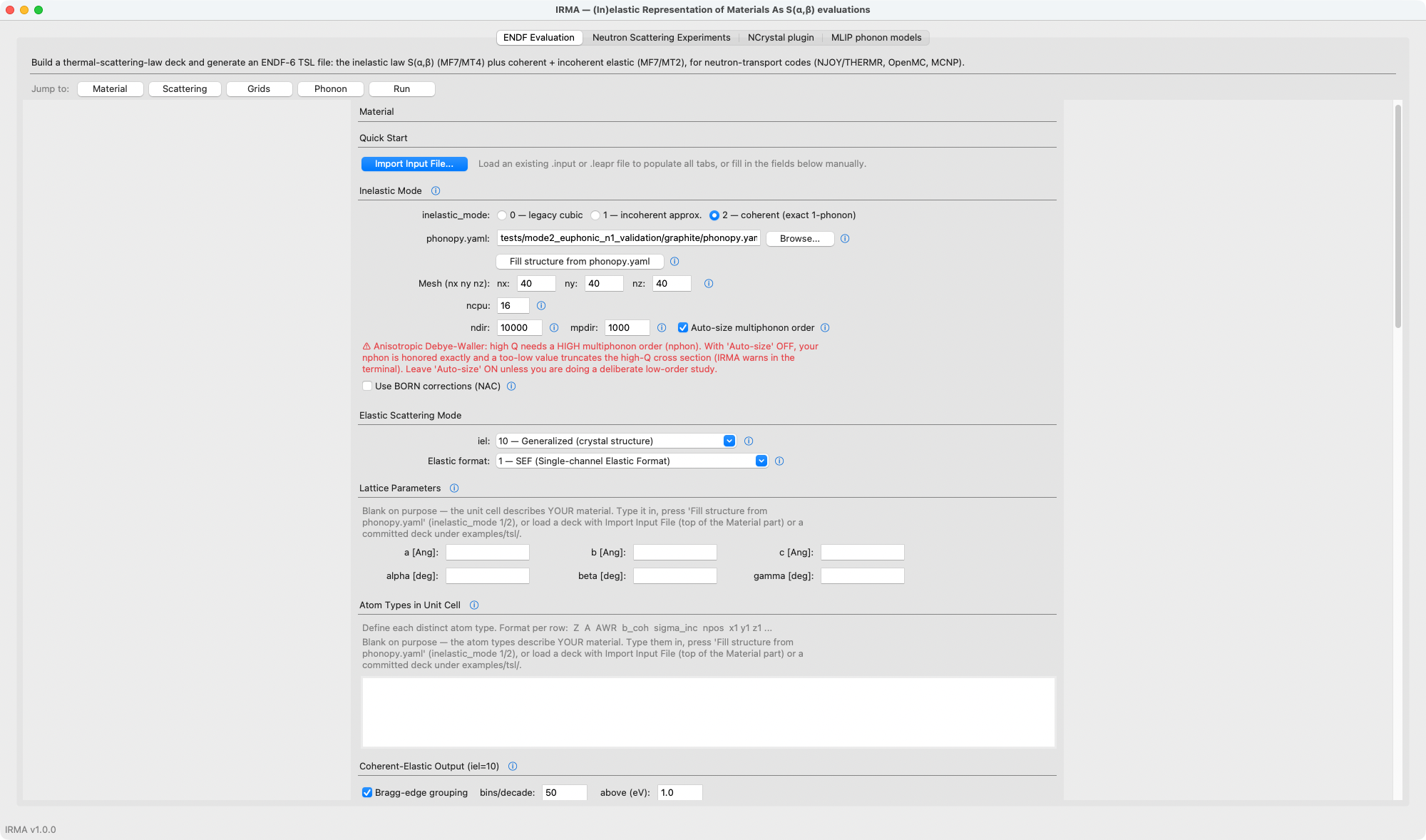
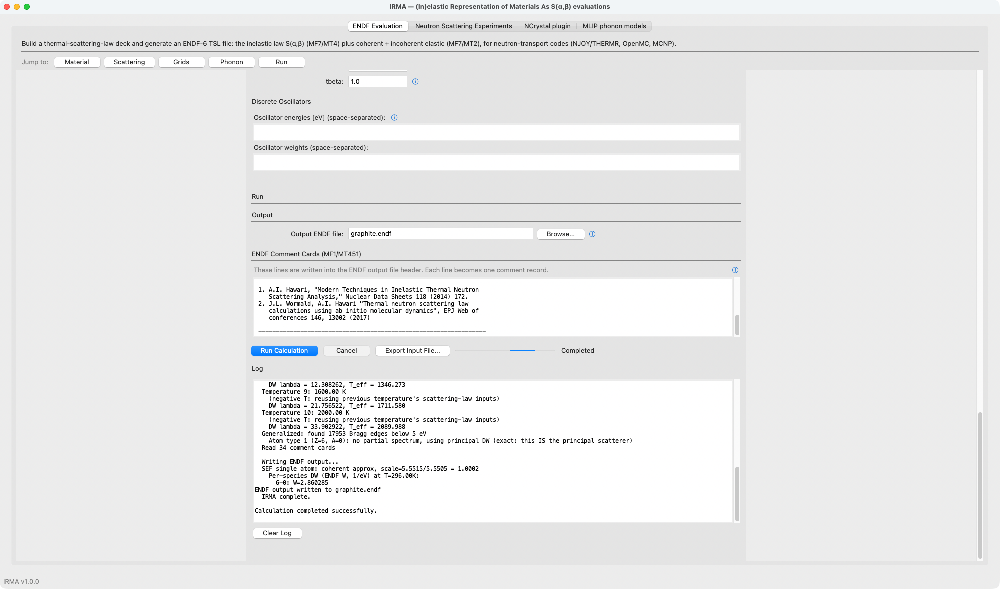
irma-gui (or python -m irma --gui) edits and runs the same input files. Use Import Input File on the ENDF Evaluation tab to load examples/tsl/graphite_mode2.input: the Material part reveals the crystal-structure and phonopy sections exactly as the input file fills them, and the Run part streams the same log shown above. A fresh form leaves the material-identity fields (ZA, MAT, AWR, sigma_free, the lattice, the atom types) blank on purpose, so importing an input file is also the quickest way to a filled form.

Processing the tape with NJOY

The tape is ready for NJOY THERMR and downstream processing. Coherent inelastic_mode=2 tapes such as this one trigger a defect in stock NJOY2016 THERMR (the cliq liquid-extrapolation guard) that produces garbage cross sections above about 0.27 eV; apply the one-line patch described in NJOY interoperability before processing. Classic and mode-1 tapes are unaffected.

Where to go from here

The scattering modes page maps the physics options this input file chose against the alternatives; the validation record shows this exact material checked against NJOY, Euphonic, OCLIMAX, and measurement; and the structure-to-spectrum tutorial starts one step earlier, from a bare crystal structure with no phonon calculation at all.