DOS-based spectra (mode 0)

The neutron scattering forward model (irma.spectra) turns a phonon calculation into an instrument-resolved 1-D inelastic neutron scattering (INS) spectrum or a 2-D S(Q,E) powder map. Its inelastic_mode selects how the inelastic scattering is computed:

Mode	Inelastic engine	Debye-Waller	Needs
0	DOS incoherent-approximation phonon expansion	isotropic (one scalar Debye-Waller factor per element)	a phonon DOS (file or phonopy)
1	phonopy eigenvectors, incoherent approximation	anisotropic (per-atom tensors)	phonopy.yaml + mesh
2	phonopy eigenvectors, coherent one-phonon + multiphonon	anisotropic	phonopy.yaml + mesh

Mode 0 is the lightweight end of the range. It runs the same incoherent-approximation phonon expansion LEAPR (NJOY's standard thermal scattering law module) uses, straight from a phonon density of states (DOS), with no eigenvectors and without the mode-1/2 engine. It is the right choice when the material is hydrogen-rich, incoherent, or disordered, where the incoherent approximation is already excellent and hydrogen dominates the signal; when a DOS is all you have, whether from molecular dynamics (via the velocity autocorrelation function), from a measurement, or from a quick calculation; or when you want a fast survey before committing to a full mode-1/2 run. It does not capture coherent inelastic scattering (phonon dispersion); use mode 2 for that. The modeling level is the same as OCLIMAX's DOS-based mode (TASK=0), but driven by IRMA's own LEAPR kernel and wired into the full instrument, resolution, and elastic forward model.

Multi-element materials

Each element scatters by its own partial DOS, mass, and Debye-Waller factor; the result is the cross-section- and multiplicity-weighted per-atom average

\[ \frac{d^2\sigma}{d\Omega\,dE'}(Q,E)=\frac{1}{N}\sum_d m_d\,\frac{\sigma_d}{4\pi}\, e^{-2W_d(Q)}\,[\text{expansion of }\rho_d],\qquad \alpha_d=\frac{C_E\,Q^2}{A_d\,k_BT}, \]

with \(C_E\) the α-conversion constant (\(\hbar^2/2m_n\)), \(A_d\) the atomic weight ratio, \(m_d\) the multiplicity, and \(N=\sum_d m_d\) the atoms per cell. The \(1/N\) makes the absolute scale per represented atom (per atom of the cell included in the calculation), the same normalization as inelastic_mode 1 and 2 (the eigenvector engine also normalizes per represented atom), so a mode-0 and a mode-1/2 spectrum are directly comparable. Hydrogen is never blended away into a single effective spectrum, and a neutron-weighted generalized DOS (GDOS) is also produced as a 1-D summary.

Where the DOS comes from (dos_source)

• file (the default): each element supplies a generic 2-column phonon DOS (frequency, intensity). The unit is meV (the default), eV, cm-1, or THz.
• phonopy: the partial DOS (and the per-element atom multiplicity) is derived from material.phonopy_yaml plus mesh, as the trace of IRMA's anisotropic DOS tensor, normalized to one phonon per atom. You still give the scattering data (awr, sigma_bound_b, …) per element.

The elastic line (optional)

Give a unit cell and mode 0 builds an elastic line from the same Debye-Waller factors the inelastic part uses. The coherent component is a set of Bragg peaks computed from your lattice, the per-element b_coh_fm, and the fractional positions (the same edge kernel the ENDF MF7/MT2 writer uses). The incoherent component is a Debye-Waller line averaged per atom over every element, \(\frac{1}{N}\sum_d m_d(\sigma_{\mathrm{inc},d}/4\pi)e^{-2W_d}\), so the hydrogen line in a CH\(_2\) material is kept even though carbon has the larger coherent length. Coherent and incoherent share the inelastic part's per-atom scale.

Leave lattice blank and the coherent Bragg peaks are skipped. With elastic_kind: both (the default) you still get the lattice-free incoherent line; set physics.elastic: false for an inelastic-only spectrum.

Configuration

material:
  temperature_K: 300.0
  # mode-0 elastic cell (omit for inelastic-only):
  lattice: [2.4612, 2.4612, 6.7079, 90.0, 90.0, 120.0]   # a,b,c,α,β,γ
  scatterers:
    - {symbol: C, sigma_bound_b: 5.551, awr: 11.898, b_coh_fm: 6.646,
       sigma_inc_b: 0.001, dos_file: c_dos.txt, dos_unit: meV, multiplicity: 4,
       positions: [[0,0,0.25],[0,0,0.75],[0.3333,0.6667,0.25],[0.6667,0.3333,0.75]]}
physics:
  inelastic_mode: 0
  dos_source: file        # or: phonopy  (then set material.phonopy_yaml + mesh)
  elastic: true
  elastic_kind: both      # both | coherent | incoherent
grid: {e_max_meV: 250.0, de_meV: 1.0, dq_max_invA: 0.1}
instrument: {geometry: vision, e_fixed_meV: 3.5}

CLI

Run a config file (irma spectra run config.yaml -o out.csv), or use the flag form directly: select --inelastic-mode 0 and put the mode-0 extras on each scatterer string as order-free key=value tokens:

SYMBOL,sigma_bound_b,awr[,b_coh_fm[,sigma_inc_b]][,dos=FILE,unit=U,mult=N,pos=x:y:z;...]

python -m irma spectra vision --inelastic-mode 0 --temperature 300 \
    --scatterer "C,5.551,11.898,6.646,0.001,dos=c_dos.txt,mult=4,pos=0:0:0.25;0:0:0.75;0.3333:0.6667:0.25;0.6667:0.3333:0.75" \
    --lattice 2.4612,2.4612,6.7079,90,90,120 -o graphite_vision.csv

--lattice (with per-scatterer pos= sites) enables the coherent-elastic Bragg peaks; --dos-source phonopy derives the partial DOS from --phonopy-yaml and --mesh instead of dos= files.

GUI

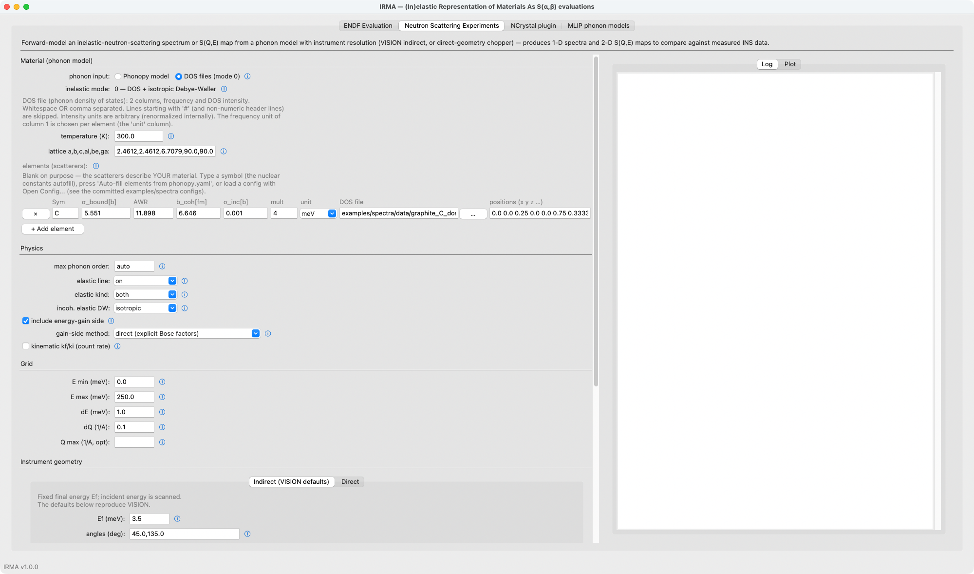
In the Neutron Scattering Experiments tab the first control, phonon input, gates everything:

• Phonopy model (the default): set inelastic mode to 0 (DOS + isotropic DW) for the DOS-derived path; the partial DOS comes from the phonopy.yaml and mesh. Auto-fill elements from phonopy.yaml populates the element table for you.
• DOS files (mode 0): the manual path, with no phonopy. Build the element table with + Add element; each row gets its own DOS file (Browse) and unit.

Fill the per-element scattering data (σ_bound, awr, b_coh, σ_inc) in the table. For the coherent-elastic line, set elastic kind to include coherent and fill the material lattice and each element's positions (flat x y z x y z …, the same format as the ENDF input file; the triplet count must equal mult).

Validation

tests/mode0_validation/validate_mode0_vs_mode1.py cross-checks mode 0 against the mode-1 engine on graphite; this is a sanity check, not a controlled proof. Because both normalize per represented atom, they agree in absolute scale (the integral ratio is ≈ 1.02) and the area-normalized shapes track closely (cosine similarity ≈ 0.92). The residual, the ~2% integral excess and the shape difference, is consistent with mode 0's isotropic Debye-Waller factor against mode 1's anisotropic one on this strongly anisotropic crystal, the same approximation OCLIMAX TASK=0 makes. A dedicated quantitative comparison against OCLIMAX TASK=0 and against measured hydrogen-rich INS spectra has not yet been performed.